一类刚弹混合碰撞系统的动力学分析

Analysis on a Kind of Rigid-Elastic Hybrid Collision System

摘要: 为了研究动力系统中同时含有刚性碰撞过程和弹性碰撞过程时的系统特性，本文给出了一类新的既含有刚性碰撞又含有弹性碰撞过程的碰撞振动模型。通过建立全局Poincaré映射的方法解析的分析了此碰撞振动系统的一周期一碰及一周期n碰的周期运动条件。数值仿真模拟了系统的周期碰撞运动现象，并得到了随参数发生变化时，系统出现的分岔现象，且利用数值仿真的方法对系统中的共存吸引子进行了初步研究。

Abstract: In order to study the system characteristics of a dynamic system with both rigid and elastic colli-sions, a new type of collisional vibration model with both rigid and elastic collisions is presented in this paper. A global Poincaré mapping method is used to analyze the conditions of one-collision- one-period and n-collisions-one-period motion vibration system. The numerical simulation simu-lates the system’s periodic collision movement phenomenon, and obtains the bifurcation phe-nomenon that occurs when the parameters change with the system. The numerical simulation method is used to study the coexistence attractors in the system.

1. 引言

碰撞振动是我们日常生活和生产实际中经常见到的一种现象，其研究涉及工程机械、工程力学、应用物理、应用数学等多个专业领域。在工程实际中，一方面，为了某种生产目的，可以利用碰撞振动的动力学原理设计制造多种冲击机械，例如，振动落砂机、冲击钻进机械、振动筛、振动锤、打桩机、微振造型机及打印机机头等。分段线性动力系统在机械中经常遇到，且由于其不连续性使得这种系统有着复杂的动力学行为。 [1] [2] [3] 详细介绍了连续动力系统的分岔与混沌。Hartog和Mikina [4] 对不含阻尼时的分段线性系统进行了研究，并得到了对称周期运动的闭形式解。Shaw和Holmes [5] 利用映射的方法研究了一类简单不连续分段线性系统的混沌运动。Nordmark [6] 通过擦边分岔研究了系统的非周期运动。Kleczka et al. [7] 研究了一类分段线性振动的周期运动和分岔，且数值仿真了系统的擦边运动。Wiercigroch [8] 给出了不连续的动力系统模型，并得到了一个关于响应的数值方法。Luo et al. [9] 得到了一种分段线性碰撞系统解的数值方法。Luo [10] 利用介于两次碰撞之间的时间间隔得到了对称的周期1运动。Albert C. J. Luo，和Santhosh Menon [11] [12] 分析了一类分段线性系统的全局周期一运动及其稳定性，以及系统的全局混沌。

机械系统中的碰撞现象分为刚性碰撞和弹性碰撞两种，关于这两类碰撞系统的研究已非常广泛，但对于一个即含有刚性碰撞同时还有弹性碰撞现象发生的系统的研究却不多见。但是这类现象在日常生活中却很多，例如火车车轮的运动等。因此对这类现象的研究是很有价值的。本文通过引入一类简单的动力学模型，试图对这类系统进行分析。

2. 力学模型

考虑一个分段线性碰撞动力系统(图1)，在这个模型中，质体M和阻尼器D相连，与弹簧C的作用有一个间隙E，质体M与刚性顶墙的距离为L，碰撞恢复系数为R。作用在质体M上的周期谐波激励为 $A\cos \Omega t$ ，其中W和A分别是激励频率和振幅。系统的运动微分方程是：

$x<L$ 时：

$M\ddot{x}+D\stackrel{\dot{}}{x}+k\left(x\right)=A\cos \Omega t$ (1)

其中： $k\left(x\right)=\{\begin{array}{l}0,x\ge -E;\\ Cx+CE,x<-E.\end{array}$

$x=L$ 时：

${\stackrel{\dot{}}{x}}_{+}=-R{\stackrel{\dot{}}{x}}_{-}$ (2)

其中 ${\stackrel{\dot{}}{x}}_{+},{\stackrel{\dot{}}{x}}_{-}$ 分别表示质体在碰撞后和碰撞前瞬时的速度。

运动方程的无量纲运动方程为：

Figure 1. Piecewise-linear impact dynamic system model

图1. 分段线性碰撞动力系统模型

$\ddot{x}+2d\stackrel{\dot{}}{x}+k\left(x\right)=a\cos \Omega t,x<L$ (3)

${\stackrel{\dot{}}{x}}_{+}=-R{\stackrel{\dot{}}{x}}_{-},x=L$ (4)

其中： $k\left(x\right)=\{\begin{array}{l}0,x\ge -E;\\ cx+e,x<-E.\end{array}$ $d=D/2M,c=C/M,e=cE,a=A/M$ 。

为了描述系统的运动情况，可以根据回复力的三个不同线性区域，以及碰撞的发生，将运动分成三个部分，即一区 $x=L$ ，二区 $-E\le x<L$ ，三区 $x\le -E$ 。对于每一个线性区，方程(3)的解可以容易求出，方程的解为：一区时发生碰撞，此时的方程为：

${\stackrel{\dot{}}{x}}_{+}=-R{\stackrel{\dot{}}{x}}_{-}$ (5)

二区中对应的微分方程是：

$\ddot{x}+2d\stackrel{\dot{}}{x}=a\cos \Omega t$ (6)

通解为：

$x=C_1+C_2{\text{e}}^{-2dt}+a{D}_1\cos \Omega t+a{D}_2\sin \Omega t$ (7)

其中 $C_1,C_2$ 是任意常数。取定初始条件 $\left(t,x,\stackrel{\dot{}}{x}\right)=\left(t_i,x_i,y_i\right)$ ，则对应的特解为：

$\begin{array}{l}x=C_1\left(t_i\right)+C_2\left(t_i\right){\text{e}}^{-2d\left(t-t_i\right)}+a\left(D_1\cos \Omega t+D_2\sin \Omega t\right)\\ \stackrel{\dot{}}{x}=-2d{C}_2\left(t_i\right){\text{e}}^{-2d\left(t-t_i\right)}-a\Omega \left(D_1\sin \Omega t-D_2\cos \Omega t\right)\end{array}$ (8)

其中：

$\begin{array}{l}{C}_1\left(t_i\right)=\frac{1}{2d}\left(y_i+2d{x}_i-\frac{a}{\Omega }\sin \Omega t_i\right),\\ C_2\left(t_i\right)=-\frac{1}{2d}\left[y_i+a\Omega \left(D_1\sin \Omega t_i-D_2\cos \Omega t_i\right)\right],\\ D_1=\frac{-1}{{\Omega }^2+4d^2},D_2=\frac{2d}{\Omega \left({\Omega }^2+4d^2\right)}\end{array}$

三区中对应的微分方程是：

$\ddot{x}+2d\stackrel{\dot{}}{x}+cx+e=a\cos \Omega t$ (9)

通解为：

$x=\left(C_3\cos \Omega t+C_4\sin \Omega t\right){\text{e}}^{-dt}-E+a\left(D_3\cos \Omega t+D_4\sin \Omega t\right)$ (10)

其中 $C_3,C_4$ 是任意常数。取定初始条件 $\left(t,x,\stackrel{\dot{}}{x}\right)=\left(t_i,x_i,y_i\right)$ ，则对应的特解为：

$\begin{array}{l}x=\left[C_3\left(t_i\right)\cos \omega \left(t-t_i\right)+C_4\left(t_i\right)\sin \omega \left(t-t_i\right)\right]{\text{e}}^{-d\left(t-t_i\right)}+a\left(D_3\cos \Omega t+D_4\sin \Omega t\right)\\ \stackrel{\dot{}}{x}=\left\{\left[C_4\left(t_i\right)\omega -C_3\left(t_i\right)d\right]\cos \omega \left(t-t_i\right)-\left[C_3\left(t_i\right)\omega +C_4\left(t_i\right)d\right]\sin \omega \left(t-t_i\right)\right\}{\text{e}}^{-d\left(t-t_i\right)}\\ -a\Omega \left(D_3\sin \Omega t-D_4\cos \Omega t\right)\end{array}$ (11)

其中：

$\begin{array}{l}{C}_3\left(t_i\right)=x_i+E-a\left(D_3\sin \Omega t_i+D_4\cos \Omega t_i\right),\\ C_4\left(t_i\right)=\frac{1}{\omega }\left[y_i+d\left(x_i+E\right)-a\left(d{D}_3+\Omega D_4\right)\cos \Omega t_i-a\left(d{D}_4-\Omega D_3\right)\sin \Omega t_i\right].\end{array}$

且 $\omega =\sqrt{c-d^2},D_3=\frac{c-{\Omega }^2}{{\left(c-{\Omega }^2\right)}^2+4d^2{\Omega }^2},D_4=\frac{2d\Omega }{{\left(c-{\Omega }^2\right)}^2+4d^2{\Omega }^2}$ 。

为了得到全局解，两个不连续交换面可以看成是映射面，即：

${\Sigma }^{+}=\left\{\left(t_i,x_i,y_i\right)|x_i=L,{\stackrel{\dot{}}{x}}_i=y_i\right\}$ 和 ${\Sigma }^{-}=\left\{\left(t_i,x_i,y_i\right)|x_i=-E,{\stackrel{\dot{}}{x}}_i=y_i\right\}$ 。 (12)

如图2所示， ${\Sigma }^{+}$ 和 ${\Sigma }^{-}$ 分别表示一区，二区，三区的分界面。两个交换面进而可以被分解为：

${\Sigma }^{+}={\Sigma }_{+}^{+}\cup {\Sigma }_{-}^{+}\cup \left\{t_i,L,0\right\}$ 和 ${\Sigma }^{-}={\Sigma }_{+}^{-}\cup {\Sigma }_{-}^{-}\cup \left\{t_i,-E,0\right\}$ ， (13)

其中：

${\Sigma }_{+}^{+}=\left\{\left(t_i,x_i,y_i\right)|x_i=L,{\stackrel{\dot{}}{x}}_i=y_i>0\right\}$ 和 ${\Sigma }_{-}^{+}=\left\{\left(t_i,x_i,y_i\right)|x_i=L,{\stackrel{\dot{}}{x}}_i=y_i<0\right\}$ ； (14)

${\Sigma }_{+}^{-}=\left\{\left(t_i,x_i,y_i\right)|x_i=-E,{\stackrel{\dot{}}{x}}_i=y_i>0\right\}$ 和 ${\Sigma }_{-}^{-}=\left\{\left(t_i,x_i,y_i\right)|x_i=-E,{\stackrel{\dot{}}{x}}_i=y_i<0\right\}$ 。 (15)

集 ${\Sigma }_{+}^{+}$ 和 ${\Sigma }_{-}^{+}$ 由点 $\left\{t_i,L,0\right\}$ 连接，集 ${\Sigma }_{+}^{-}$ 和 ${\Sigma }_{-}^{-}$ 由点 $\left\{t_i,-E,0\right\}$ 连接。两个奇点之间的运动直接与外力有关，两个奇点之间的运动是在两个交换面之间从一端到另一端。

3. 一周期一碰和一周期n碰周期运动及其稳定性

为了研究一周期一碰运动，我们可以首先基于两个交换面的四个子集，建立四个映射：

$P_1:{\Sigma }_{-}^{+}\to {\Sigma }_{-}^{-},P_2:{\Sigma }_{-}^{-}\to {\Sigma }_{+}^{-},P_3:{\Sigma }_{+}^{-}\to {\Sigma }_{+}^{+},P_4:{\Sigma }_{+}^{+}\to {\Sigma }_{-}^{+}$ (16)

在区域一中映射 $P_1$ 将状态 $\left(t_i,L,y_i\right)$ $\left(y_i<0\right)$ 映射成另一个状态 $\left(t_{i+1},-E,y_{i+1}\right)$ $\left(y_{i+1}<0\right)$ ，其它映射也如图2所示。四个映射的表达式很容易给出。

利用Poincaré映射 $P:{\Sigma }_{-}^{+}\to {\Sigma }_{-}^{+}$ ，可以分析全局一周期一碰运动。映射关系如图3所示，Poincaré映射为：

$P=P_4\circ P_3\circ P_2\circ P_1$ (17)

根据方程(10)，对于点 $\left(t_i,L,y_i\right)\in {\Sigma }_{-}^{+}$ ，有如下映射关系：

$\begin{array}{l}{P}_1:\left(t_i,L,y_i\right)\to \left(t_{i+1},-E,y_{i+1}\right),\\ P_2:\left(t_{i+1},-E,y_{i+1}\right)\to \left(t_{i+2},-E,y_{i+2}\right),\\ P_3:\left(t_{i+2},-E,y_{i+2}\right)\to \left(t_{i+3},L,y_{i+3}\right),\\ P_4:\left(t_{i+3},L,y_{i+3}\right)\to \left(t_{i+4},L,y_{i+4}\right).\end{array}\}$ (18)

Figure 2. Mapping

图2. 映射指向图

Figure 3. The mapping relationship

图3. 映射关系

从方程(10)和(11)，可得

$P_4\circ P_3\circ P_2\circ P_1:\left(t_{i}L,y_i\right)\to \left(t_{i+4},L,y_{i+4}\right)$ (19)

一周期一碰的周期运动的条件为

$t_{i+4}=t_i+T,y_{i+4}=y_i$ (20)

映射 $P_1:\left(t_i,L,y_i\right)\to \left(t_{i+1},-E,y_{i+1}\right)$ 由下列方程组决定：

$\begin{array}{l}E+C_1\left(t_i\right)+C_2\left(t_i\right){\text{e}}^{-2d\left(t_{i+1}-t_i\right)}+a\left(D_1\cos \Omega t_{i+1}+D_2\sin \Omega t_{i+1}\right)=0,\\ y_{i+1}+2d{C}_2\left(t_i\right){\text{e}}^{-2d\left(t_{i+1}-t_i\right)}+a\Omega \left(D_1\sin \Omega t_{i+1}-D_2\cos \Omega t_{i+1}\right)=0.\end{array}$ (21)

映射 $P_2:\left(t_{i+1},-E,y_{i+1}\right)\to \left(t_{i+2},-E,y_{i+2}\right)$ 由下列方程决定：

$\begin{array}{l}E+\left[C_3\left(t_{i+1}\right)\cos \omega \left(t_{i+2}-t_{i+1}\right)+C_4\left(t_{i+1}\right)\sin \omega \left(t_{i+2}-t_{i+1}\right)\right]{\text{e}}^{-d\left(t_{i+2}-t_{i+1}\right)}\\ +a\left(D_3\cos \Omega t_{i+2}+D_4\sin \Omega t_{i+2}\right)=0,\\ y_{i+2}-\{\left[C_4\left(t_{i+1}\right)\omega -C_3\left(t_{i+1}\right)d\right]\cos \omega \left(t_{i+2}-t_{i+1}\right)\\ -\left[C_3\left(t_{i+1}\right)\omega +C_4\left(t_{i+1}\right)d\right]\sin \omega \left(t_{i+2}-t_{i+1}\right)){\text{e}}^{-d\left(t_{i+2}-t_{i+1}\right)}\\ +a\Omega \left(D_3\sin \Omega t_{i+2}-D_4\cos \Omega t_{i+2}\right)=0.\end{array}$ (22)

映射 $P_3:\left(t_{i+2},-E,y_{i+2}\right)\to \left(t_{i+3},L,y_{i+3}\right)$ 由下列方程决定：

$\begin{array}{l}L-C_1\left(t_{i+2}\right)-C_2\left(t_{i+2}\right){\text{e}}^{-2d\left(t_{i+3}-t_{i+2}\right)}-a\left(D_1\cos \Omega t_{i+3}+D_2\sin \Omega t_{i+3}\right)=0,\\ y_{i+3}+2d{C}_2\left(t_{i+2}\right){\text{e}}^{-2d\left(t_{i+3}-t_{i+2}\right)}+a\Omega \left(D_1\sin \Omega t_{i+3}-D_2\cos \Omega t_{i+3}\right)=0.\end{array}$ (23)

映射 $P_4:\left(t_{i+3},L,y_{i+3}\right)\to \left(t_{i+4},L,y_{i+4}\right)$ 由下列方程决定：

$\begin{array}{l}{t}_{i+4}=t_{i+3},\\ y_{i+4}=-R{y}_{i+3}.\end{array}$ (24)

解方程组(13)~(17)可得一周期一碰的分析解。一周期一碰的周期解的稳定性可以通过Poincaré映射的Jacobian矩阵来分析。由方程(10)和(11)，Jacobian矩阵可以通过链式法则表示为：

$DP={\left[\frac{\partial \left(t_{i+4},y_{i+4}\right)}{\partial \left(t_i,y_i\right)}\right]}_{\left(t_i,y_i\right)}={\displaystyle \underset{j=1}{\overset{4}{\prod }}D{P}_j}={{\displaystyle \underset{j=1}{\overset{4}{\prod }}\left[\frac{\partial \left(t_{i+j},y_{i+j}\right)}{\partial \left(t_{i+j-1},y_{i+j-1}\right)}\right]}}_{\left(t_{i+j-1},y_{i+j-1},t_{i+j},y_{i+j}\right)}$ (25)

通过对Poincaré映射的特征值的分析，就能得到周期运动的稳定行，即若特征值的实部均小于零时，则周期运动稳定，否则，不稳定。

对于一周期n碰的周期运动，根据一周期一碰的运动情况，为了描述一周期n碰，我们只需要在交换面 ${\Sigma }^{+}$ 上进一步给出映射 $P_5$ (图4)，根据一周期一碰的Poincaré映射建立的方法，我们可以进一步得到一周期n碰的Poincaré映射。图5给出了对应的映射关系图。

因而对应的Poincaré映射为：

$P=P_4{\left(P_5{P}_4\right)}_{n-1}{P}_3{P}_2{P}_1$

其中 ${\left(P_5{P}_4\right)}_{n-1}$ 表示 $P_5{P}_4$ 的 $n-1$ 次复合。

4. 数值仿真

利用Mathematica数学软件，对于系统的碰撞情况根据(21)、(22)、(23)、(24)进行了仿真，在交换面处控制精度小于0.001。在其它参数不变的条件下，随着激励力振幅a的增大，系统碰撞(指质体M与刚性顶墙的碰撞)次数增加，出现从一周期一碰到一周期二碰，及一周期多碰的现象。随参数a的变化，系统关于碰撞次数出现加1分岔。

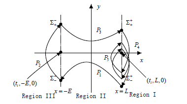
Figure 4. One-period of n collision mapping

图4. 一周期n碰映射图

Figure 5. Mapping diagram

图5. 映射关系图

图6给出了当参数分别取 $E=1;L=1;c=0.5;e=0.5;\Omega =0.55;d=0.05;r=0.8$ 时系统关于参数a发生碰撞的次数(6—1)及相应的Poincaré映射图。由图可知此时，当 $a<0.123$ 时，系统不发生碰撞；当 $a\ge 0.123$ 时系统发生碰撞，且当 $0.123\le a\le 1.431$ 时，系统出现稳定的一周期一碰现象； $a\ge 1.432$ 时，系统出现一周期二碰。

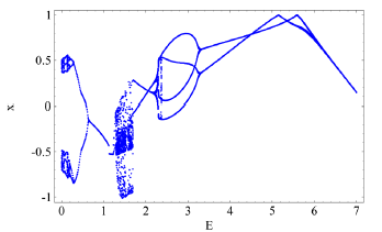
图7给出了系统在参数分别取 $L=1;c=0.9;\Omega =0.55;d=0.05;r=0.8$ 时系统关于弹性碰撞间隙E的Poincaré映射图。从Poincaré映射图可以得到，随着弹性碰撞间隙E的减小，系统出现了连续的倍周期到混沌分岔现象。图8给出了四种不同间隙E时系统运动的像图，(8-1)是当 $E=1.5$ 时系统出现的混沌运动的像图；(8-2)是当 $E=2$ 时系统出现的二周期二碰运动的像图；(8-3)是当 $E=3$ 时系统出现的四周期四碰运动的像图；(8-4)是当 $E=4$ 时系统出现的二周期二碰运动的像图。

5. 共存吸引子

下面利用胞映射的方法研究系统出现的共存吸引子，首先在系统的参数分别为 $E=1;L=1;c=0.5;e=0.5;\Omega =0.55;d=0.05;r=0.8;a=0.14$ 时，系统存在两种周期一运动，其一为周期一一碰运动，另一运动为无碰撞的周期一运动。图9给出了此时系统中存在的两个共存吸引子的吸引域，

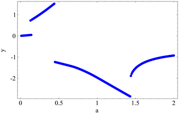(6-1) (6-2)

Figure 6. System with $E=1;L=1;c=0.5;e=0.5;\Omega =0.55;d=0.05;r=0.8$ about a (1) collision frequency map (2) Poincaré mapping

图6. 系统在参数分别取 $E=1;L=1;c=0.5;e=0.5;\Omega =0.55;d=0.05;r=0.8$ 时关于参数a的(1) 碰撞次数图 (2) Poincaré映射图

(7-1) (7-2)

Figure 7. Mapping of system with $L=1;c=0.9;\Omega =0.55;d=0.05;a=1;r=0.8$ about E (1) Displacement (2) Velocity Poincaré

图7. 系统在参数分别取 $L=1;c=0.9;\Omega =0.55;d=0.05;a=1;r=0.8$ 时关于弹性碰撞间隙E的(1) 关于位移 (2) 关于速度的Poincaré映射图

(8-1) (8-2) (8-3) (8-4)

Figure 8. Phase diagram of system with $L=1;c=0.9;\Omega =0.55;d=0.05;a=1;r=0.8$ (1) $E=1.5$ ; (2) $E=2$ ；(3) $E=3$ ; (4) $E=4$

图8. 系统在参数分别取 $L=1;c=0.9;\Omega =0.55;d=0.05;a=1;r=0.8$ ；(1) $E=1.5$ ；(2) $E=2$ ；(3) $E=3$ ；(4) $E=4$ 时的相图

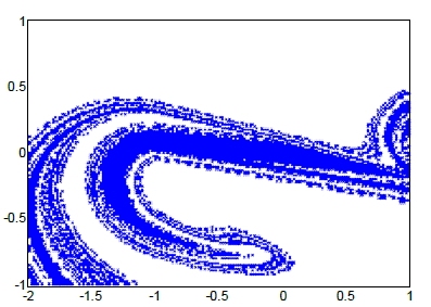
Figure 9. Coexisting attractor domain of system with parameters $E=1;L=1;c=0.5;e=0.5;\Omega =0.55;d=0.05;r=0.8;a=0.14$

图9. 系统在参数分别取 $E=1;L=1;c=0.5;e=0.5;\Omega =0.55;d=0.05;r=0.8;a=0.14$ 时共存吸引子的吸引域

其中蓝色区域为一周期一碰运动的吸引域，白色区域为周期一运动的吸引域。图10分别给出了这两种运动状态在初始点分别为 $\left(0,-0.5\right),\left(0.5,0\right)$ 时的系统稳定时的相图。在系统的参数分别为 $E=1;L=1;c=0.5;e=0.5;\Omega =0.55;d=0.05;r=0.8;a=1.44$ 时，系统存在两种周期一运动，其一为周期一一碰运动，另一运动为周期一二碰运动，图11给出了此时系统中存在的两个共存吸引子的吸引域，其中蓝色区域为一周期二碰运动的吸引域，白色区域为一周期一碰运动的吸引域。图12分别给出了这两种运动状态在初始点分别为 $\left(-2,0\right),\left(0,4\right)$ 时的系统稳定时的相图。

(10-1) (10-2)

Figure 10. Phase diagram of system with $E=1;L=1;c=0.5;e=0.5;\Omega =0.55;d=0.05;r=0.8;a=0.14$ (1) Initial point $\left(0,-0.5\right)$ (2) Initial point $\left(0.5,0.5\right)$

图10. 系统在参数分别取 $E=1;L=1;c=0.5;e=0.5;\Omega =0.55;d=0.05;r=0.8;a=0.14$ 时的相图，(1) 初始点为 $\left(0,-0.5\right)$ ；(2) 初始点为 $\left(0.5,0.5\right)$

Figure 11. Coexisting attractor domain of system with parameters $E=1;L=1;c=0.5;e=0.5;\Omega =0.55;d=0.05;r=0.8;a=1.44$

图11. 系统在参数分别取 $E=1;L=1;c=0.5;e=0.5;\Omega =0.55;d=0.05;r=0.8;a=1.44$ 时共存吸引子的吸引域

(12-1) (12-2)

Figure 12. Phase diagram of system with $E=1;L=1;c=0.5;e=0.5;\Omega =0.55;d=0.05;r=0.8;a=1.44$ (1) Initial point $\left(-2,0\right)$ (2) Initial point $\left(0,4\right)$

图12. 系统在参数分别取 $E=1;L=1;c=0.5;e=0.5;\Omega =0.55;d=0.05;r=0.8;a=1.44$ 时的相图(1) 初始点为 $\left(-2,0\right)$ ；(2) 初始点为 $\left(0,4\right)$

6. 结论

本文考虑了一类分段线性碰撞系统的动力学行为，当取定交换面为Poincaré截面时，给出了一周期一碰及一周期n碰的具体的Poincaré映射，由此可以解析的分析其周期运动的稳定性。虽然每一段Poincaré映射的解析表达式可以给出，但由于对其进行复合的过程难以解析的实现，因此，本文仅给出了具体的Poincaré映射构造的途径和方法。如果需要进一步讨论的话，就需要对系统本身作进一步的改造或提出新的理论基础。进而利用数值仿真的方法对系统的分岔现象进行了说明。并利用胞映射的方法对系统的共存吸引子进行了研究，得到了一些结论。

基金项目：

河南省教育厅省重大科技攻关计划项目：非光滑动力系统的理论及应用研究(14B130001)。

参考文献