关于时间慢变的广义Logistic模型的多尺度分析

doi:10.12677/AAM.2018.77112

期刊菜单

关于时间慢变的广义Logistic模型的多尺度分析
Multiscale Analysis of a Generalized Logistic Model with Slowly Varying Parameters

DOI: 10.12677/AAM.2018.77112, PDF, HTML, XML, 下载: 1,018 浏览: 2,199
作者: 李磊, 谢峰：东华大学理学院，上海
关键词: 多尺度；广义logistic模型；慢变参数；渐近解；Multi-Scale； The Generalized Logistic Model； Asymptotic Solution； Slowly Varying Parameters

摘要: 在广义logistic模型中，有三个参数，分别为R (种群内禀增长率)，K (种群最大容纳量)，β (种群对环境利用程度的参数)。模型中它们通常为常数，但在自然环境中它们都是关于时间缓慢变化的，这时模型的精确解是求不出来的。本文通过使用多尺度的方法求出关于时间慢变模型的渐近解，数值模拟例证了所得渐近解的有效性。

Abstract: In the generalized logistic model, there are three parameters, R (intrinsic rate of growth), K (maxi-mum tolerance of population) and β (the degree of population using environmental resources), which are constants in the model. In fact, they vary slowly with time in the natural environment. It is hard to obtain the exact solution. In this paper we get the asymptotic solution of the model using the method of multi-scale. Numerical simulation illustrates the validity of the asymptotic solution obtained.

文章引用：李磊, 谢峰. 关于时间慢变的广义Logistic模型的多尺度分析[J]. 应用数学进展, 2018, 7(7): 956-961. https://doi.org/10.12677/AAM.2018.77112

1. 引言

在单种群生态学中，许多学者相继提出了很多模型用来刻画单种群的增长规律，经典的单种群模型有Malthus模型、Logistic模型等。1963年，Smith在研究大型水蚤的种群增长时提出了较为广义的Logistic模型 [1] ：

$\frac{d M}{M d T} = R (\frac{K - M}{K + (R / C) M}),$ (1)

其中，M为种群的规模(实际上为水蚤重量)，K为种群能够达到的饱和值，R为资源充足时种群的增长率，C为饱和状态下种群规模的置换率。1990年，王寿松等 [2] [3] 对模型(1)进行了深入研究，(1)所描述的生物增长曲线与Logistic模型显著不同，同样具有研究价值。

考虑到实际问题中参数一般随时间是缓慢变化的，本文研究如下关于时间慢变的广义logistic模型：

$\frac{d X}{d T} = \frac{R (T) X (1 - \frac{X}{K (T)})}{1 + ε \bar{β} (T) X}, X (0) = X_{0} .$ (2)

模型中 $R, K, \bar{β}$ 随时间慢变的，即 $R (ε t), K (ε t), \bar{β} (ε t)$ ，t为时间， $ε$ 为小的正参数。此时难以求出问题(2)的精确解，我们用多尺度方法研究问题(2)的渐近解。

近年来，国内外有很多学者将奇摄动理论应用于关于时间慢变带有小参数单种群模型。2007年，T. Grozdanovski使用多尺度方法研究了参数慢变Gompertz模型 [4] 。2009年至2016年，M. A. Idlango, T. Grozdanovski [5] [6] [7] [8] 等也用同样的方法对几类logistic模型做了深入研究。同样，国内也有学者在这个方向进行了深入探讨。2013年，Jianhe Shen [9] [10] 用匹配法构造了带有收获项的Logistic方程的渐近解。2016年，聂冬冬 [11] 通过合成展开法得到了带有Allee效应的广义Logistic方程的渐近解。

在对(2)做多尺度分析之前，需要将参数无量纲化：

$K (ε t) = K_{0} k (ε t), \bar{β} (ε t) = β_{0} β (ε t), R (ε t) = R_{0} r (ε t),$ (3)

(2)式变换为

$\frac{d x (t, ε)}{d t} = \frac{r (ε t) x (1 - \frac{x (t, ε)}{k (ε t)})}{1 + ε σ β (ε t) x (t, ε)}, x (0, ε) = μ .$ (4)

其中 $σ = β_{0} K_{0}, μ = \frac{X_{0}}{K_{0}}$ ，

在(4)中各部分存在不同时间的变化，我们能够应用多尺度方法于(4)并构造其在 $t \geq 0$ 都有效的形式渐近解。

2. 多尺度分析

模型(4)依赖于两个时间尺度，普通时间t与慢时间 $ε t$ ，考虑到这个特征，作广义的两时间尺度变换：

$t_{0} = \frac{1}{ε} g (t_{1}), t_{1} = ε t,$ (5)

$t_{1}$ 相对于 $t_{0}$ 为慢时间尺度，且需满足 $g (t_{1}) > 0 (t_{1} > 0), g (0) = 0$ ，这里 $r, k, \bar{β}$ 都变为关于 $t_{1}$ 的函数 $r (t_{1}), k (t_{1}), \bar{β} (t_{1})$ 。此外，为了让 $t_{0}$ 与 $t_{1}$ 一一对应，我们需要假定 $g^{'} (t_{1}) > 0$ 。

将 $x (t, ε)$ 看作两个时间尺度的函数 $x (t_{0}, t_{1}, ε)$ ，再运用链式法则得到的多尺度等式

$g^{'} (t_{1}) D_{0} x (t, ε) + ε D_{1} x (t, ε) = \frac{r (ε t) x (1 - \frac{x (t, ε)}{k (ε t)})}{1 + ε σ β (ε t) x (t, ε)},$ (6)

其中 $D_{0} x = \frac{\partial x}{\partial t_{0}}, D_{1} x = \frac{\partial x}{\partial t_{1}}$ 。

显然(6)式为x关于 $t_{0}$ 、 $t_{1}$ 的偏微分方程，常微分方程(4)与偏微分方程(6)是等价的。接下来，对(6)进行摄动分析，假定x关于 $ε$ 的庞加莱展开式为以下形式：

$x (t_{0}, t_{1}, ε) = x_{0} (t_{0}, t_{1}) + ε x_{1} (t_{0}, t_{1}) + ε^{2} x_{2} (t_{0}, t_{1}) + \dots,$ (7)

将(7)代入(6)式，可得：

$\begin{array}{l} g^{'} (t_{1}) D_{0} [x_{0} (t_{0}, t_{1}) + ε x_{1} (t_{0}, t_{1}) + ε^{2} x_{2} (t_{0}, t_{1}) + \dots] + ε D_{1} [x_{0} (t_{0}, t_{1}) + ε x_{1} (t_{0}, t_{1}) + ε^{2} x_{2} (t_{0}, t_{1}) + \dots] \\ = \frac{r (ε t) (x_{0} (t_{0}, t_{1}) + ε x_{1} (t_{0}, t_{1}) + ε^{2} x_{2} (t_{0}, t_{1}) + \dots) (1 - \frac{x_{0} (t_{0}, t_{1}) + ε x_{1} (t_{0}, t_{1}) + ε^{2} x_{2} (t_{0}, t_{1}) + \dots}{k (ε t)})}{1 + ε σ β (ε t) (x_{0} (t_{0}, t_{1}) + ε x_{1} (t_{0}, t_{1}) + ε^{2} x_{2} (t_{0}, t_{1}) + \dots)} . \end{array}$ (8)

比较关于 $ε^{0}$ 和 $ε^{1}$ 系数有

$g^{'} (t_{1}) D_{0} x_{0} = r (t_{1}) x_{0} (1 - \frac{x_{0}}{k (t_{1})});$ (9)

$g^{'} (t_{1}) D_{0} x_{1} + D_{1} x_{0} = \frac{r (t_{1})}{k (t_{1})} [x_{1} (k (t_{1}) - 2 x_{0})] - \frac{r (t_{1})}{k (t_{1})} σ β (t_{1}) [x_{0}^{2} (k (t_{1}) - x_{0})],$ (10)

同理也可以得到关于 $x_{2}, x_{3}, x_{4}$ 的方程。

解偏微分方程(9)，易得

$x_{0} = \frac{k (t_{1})}{1 + c (t_{1}) k (t_{1}) e^{- θ (t_{1}) t_{0}}},$ (11)

其中， $c (t_{1})$ 为关于 $t_{1}$ 任意函数， $θ (t_{1}) = \frac{r (t_{1})}{g^{'} (t_{1})}$ 为关于 $t_{1}$ 正函数。

利用常数变易公式，可以得到线性微分方程(10)一个特解

$\begin{matrix} x_{1} = \frac{- θ (t_{1}) σ β (t_{1}) k {(t_{1})}^{3} c (t_{1}) [t_{0} + \frac{1}{θ (t_{1})} \ln (1 + c (t_{1}) k (t_{1}) e^{- θ (t_{1}) t_{0}})]}{e^{θ (t_{1}) t_{0}} {(1 + c (t_{1}) k (t_{1}) e^{- θ (t_{1}) t_{0}})}^{2}} \\ + \frac{- \frac{k^{'} (t_{1})}{θ (t_{1})} + k {(t_{1})}^{2} c^{'} (t_{1}) t_{0} e^{- θ (t_{1}) t_{0}} - \frac{1}{2} c (t_{1}) k {(t_{1})}^{2} θ^{'} (t_{1}) t_{0}^{2} e^{- θ (t_{1}) t_{0}}}{g^{'} (t_{1}) {(1 + c (t_{1}) k (t_{1}) e^{- θ (t_{1}) t_{0}})}^{2}} . \end{matrix}$ (12)

将(11) (12)作为 $x (t_{0}, t_{1}, ε)$ 的前两项代入，可表示为

$\begin{matrix} x (t_{0}, t_{1}, ε) = \frac{k (t_{1})}{1 + c (t_{1}) k (t_{1}) e^{- θ (t_{1}) t_{0}}} \\ + ε \frac{- \frac{k^{'} (t_{1})}{θ (t_{1})}}{g^{'} (t_{1}) {(1 + c (t_{1}) k (t_{1}) e^{- θ (t_{1}) t_{0}})}^{2}} \\ + ε \frac{- σ β (t_{1}) k {(t_{1})}^{3} c (t_{1}) \ln (1 + c (t_{1}) k (t_{1}) e^{- θ (t_{1}) t_{0}})}{e^{θ (t_{1}) t_{0}} {(1 + c (t_{1}) k (t_{1}) e^{- θ (t_{1}) t_{0}})}^{2}} . \end{matrix}$ (13)

为消去长期项，令 $t_{0}^{2} e^{- θ (t_{1}) t_{0}}$ 与 $t_{0} e^{- θ (t_{1}) t_{0}}$ 的系数分别为零，即

$θ^{'} (t_{1}) = 0, \frac{c^{'} (t_{1})}{g^{'} (t_{1})} - σ θ (t_{1}) β (t_{1}) k (t_{1}) c (t_{1}) = 0 .$ (14)

特别地，令 $θ (t_{1}) = 1$ ，则有 $g^{'} (t_{1}) = r (t_{1}) (t_{1} > 0)$ ，由(7)得出 $t_{0}$

$t_{0} = \frac{1}{ε} \int_{0}^{ε t} r (s) d s .$ (15)

由(14)知 $c (t_{1}) = d e^{σ \int β (t_{1}) k (t_{1}) r (t_{1}) d t_{1}}$ ，d为任意常数。

将 $x_{0}$ 与 $x_{1}$ 代入 $x (t_{0}, t_{1}, ε)$ ，并将初值条件代入可得

$d = \frac{k (0) - μ}{μ k (0)}, c = \frac{k (0) - μ}{μ k (0)} e^{σ \int β (t_{1}) k (t_{1}) r (t_{1}) d t_{1}} .$ (16)

再由

$θ = 1, c = \frac{k (0) - μ}{μ k (0)} e^{σ \int β (t_{1}) k (t_{1}) r (t_{1}) d t_{1}},$ (17)

那么， $x (t_{0}, t_{1}, ε)$ 可以近似的表示为

$\begin{matrix} x (t_{0}, t_{1}, ε) = \frac{k (t_{1})}{1 + \frac{k (0) - μ}{μ k (0)} e^{σ \int β (t_{1}) k (t_{1}) r (t_{1}) d t_{1}} k (t_{1}) e^{- t_{0}}} \\ + ε \frac{- σ β (t_{1}) k {(t_{1})}^{3} \frac{k (0) - μ}{μ k (0)} e^{σ \int β (t_{1}) k (t_{1}) r (t_{1}) d t_{1}} \ln (1 + \frac{k (0) - μ}{μ k (0)} e^{σ \int β (t_{1}) k (t_{1}) r (t_{1}) d t_{1}} k (t_{1}) e^{- t_{0}})}{e^{θ (t_{1}) t_{0}} {(1 + \frac{k (0) - μ}{μ k (0)} e^{σ \int β (t_{1}) k (t_{1}) r (t_{1}) d t_{1}} k (t_{1}) e^{- t_{0}})}^{2}} \\ + ε \frac{- k^{'} (t_{1})}{r (t_{1}) {(1 + \frac{k (0) - μ}{μ k (0)} e^{σ \int β (t_{1}) k (t_{1}) r (t_{1}) d t_{1}} k (t_{1}) e^{- t_{0}})}^{2}} . \end{matrix}$ (18)

这样我们构造出了微分方程(6)的渐近解，因为微分方程(4)与微分方程(6)是等价的，所以，同样由(5)可构造出(4)式的形式渐近解

$\begin{matrix} x (t, ε) = \frac{k (ε t)}{1 + \frac{k (0) - μ}{μ k (0)} e^{σ ε \int β (ε t) k (ε t) r (ε t) d t} k (ε t) e^{- \frac{1}{ε} \int_{0}^{ε t} r (s) d s}} \\ + ε \frac{- σ β (ε t) k {(ε t)}^{3} \frac{k (0) - μ}{μ k (0)} e^{σ ε \int β (ε t) k (ε t) r (ε t) d t} \ln (1 + \frac{k (0) - μ}{μ k (0)} e^{σ ε \int β (ε t) k (ε t) r (ε t) d t} k (ε t) e^{- \frac{1}{ε} \int_{0}^{ε t} r (s) d s})}{e^{t_{0}} {(1 + \frac{k (0) - μ}{μ k (0)} e^{σ ε \int β (ε t) k (ε t) r (ε t) d t} k (ε t) e^{- \frac{1}{ε} \int_{0}^{ε t} r (s) d s})}^{2}} \\ + ε \frac{- k^{'} (ε t)}{r (ε t) {(1 + \frac{k (0) - μ}{μ k (0)} e^{σ ε \int β (ε t) k (ε t) r (ε t) d t} k (ε t) e^{- \frac{1}{ε} \int_{0}^{ε t} r (s) d s})}^{2}} . \end{matrix}$ (19)

3. 数值模拟

我们已通过多尺度方法得到的微分方程(4)的一阶渐近解(19)，下面需要验证它是一致有效的。在自然环境中模型(4)的三个参数 $r, k, β$ 不是常数，而是随着时间缓慢变化的。因此，(4)式没有精确解，我们需要数值模拟进行对比。在 $σ = 1$ 的情况下，由于为慢变的，分别令

$\begin{array}{l} r (ε t) = \frac{9}{10} + \frac{2}{10} \sin ε t ， \\ k (ε t) = 1 + \frac{2}{10} \sin ε t ， \\ β (ε t) = \frac{1}{2} + \frac{2}{10} \sin ε t, \end{array}$

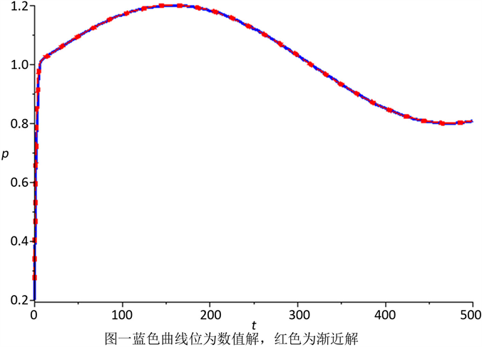
Figure 1. Curve: Comparison between the numerical solution and the asymptotic solution

图1. 数值解与渐近解的对比图

$ε = \frac{1}{100}, μ = \frac{2}{10}$ 。那么，我们可以得到模型(4)的渐近解与数值解，由图1所示，蓝色曲线(数值解)与红色的点组成的曲线(形式渐近解)在 $t \geq 0$ 时，是完全吻合的。

参考文献

[1]	Smith, F.E. (1963) Population Dynamics in Daphnia magna and a New Model for Population Growth. Ecology, 44, 651-663. https://doi.org/10.2307/1933011
[2]	王寿松. 单种群生长的广义Logistic模型[J]. 生物数学学报, 1990(1): 21-25.
[3]	李清, 王克, 范猛. 广义Logistic模型的捕获优化问题[J]. 生物数学学报, 2000, 15(4): 408-412.
[4]	Grozdanovski, T. and Shepherd, J.J. (2007) Slow Variation in the Gompertz Model. ANZIAM Journal Electronic Supplement, 47, 541-554. https://doi.org/10.21914/anziamj.v47i0.1061
[5]	Idlango, M.A., Shepherd, J.J., Nguyen, L., et al. (2012) Harvesting a Logistic Population in a Slowly Varying Environment. Applied Mathematics Letters, 25, 81-87. https://doi.org/10.1016/j.aml.2011.07.015
[6]	Idlango, M.A., Shepherd, J.J. and Gear, J.A. (2017) Logistic Growth with a Slowly Varying Holling Type II Harvesting Term. Communications in Nonlinear Science & Numerical Simulation, 49, 81-92. https://doi.org/10.1016/j.cnsns.2017.02.005
[7]	Grozdanovski, T., Shepherd, J.J. and Stacey, A. (2009) Multi-Scaling Analysis of a Logistic Model with Slowly Varying Coefficients. Applied Mathematics Letters, 22, 1091-1095. https://doi.org/10.1016/j.aml.2008.10.002
[8]	Idlango, M.A., Gear, J.A. and Shepherd, J.J. (2013) Survival to Extinction in a Slowly Varying Harvested Logistic Population Model. Applied Mathematics Letters, 26, 1035-1040. https://doi.org/10.1016/j.aml.2013.05.003
[9]	Shen, J. and Zhou, Z. (2014) Fast-Slow Dynamics in First-Order Initial Value Problems with Slowly Varying Parameters and Application to a Harvested Logistic Model. Communications in Nonlinear Science & Numerical Simulation, 19, 2624-2631. https://doi.org/10.1016/j.cnsns.2013.12.035
[10]	Shen, J. and Zhou, Z. (2013) Fast-Slow Dynamics in Logistic Models with Slowly Varying Parameters. Communications in Nonlinear Science & Numerical Simulation, 18, 2213-2221. https://doi.org/10.1016/j.cnsns.2012.12.036
[11]	聂冬冬, 谢峰. 一类具有Allee效应的Logistic模型的渐近解[J]. 应用数学, 2016(3): 678-685.

为你推荐

友情链接