基于贝塞尔多项式的第二类非线性Volterra积分方程的改进配置解法

An Improved Collocation Method for the Second Kind of Nonlinear Volterra Integral Equation Based on Bessel Polynomials

摘要: 本文提出了一种基于贝塞尔多项式的第二类非线性Volterra积分方程的配置解法，并对该方法进行了误差和收敛性分析。通过数值实例验证了该方法的有效性和适用性，并与已有的结果进行了比较，证明了其数值方法的优越性。

Abstract: In this paper, a collocation method for the second kind of nonlinear Volterra integral equation based on Bessel polynomials is proposed, and the error and convergence of the method are analyzed. The effectiveness and applicability of the method are verified by numerical examples, and the superiority of the numerical method is proved by comparing with the existing results.

1. 引言

在科学与工程计算中，非线性积分方程一直是人们研究的热点问题之一。近年来，越来越多的研究者提出了一些数值求解积分方程和积–微分方程的方法，如同伦摄动法 [1] [2]、改进的同伦摄动法 [3]、Haar函数法 [4] [5]、差分变换法 [6]，Tau方法 [7]、变分迭代法 [8]、Legendre-matrix法 [9]、Adomian法 [10] 和Galerkin法 [11] 等。Sezer等人 [12] [13] 利用Chebyshev多项式方法和Taylor配置法找到了线性微分方程及积分–微分方程组的解；此外，泰勒展开法 [14] 也是一种求解积分和积–微分方程的有效方法。 [15] - [20] 中，Huang等人利用Taylor、Chebyshev和Legendre矩阵方法求解线性Fredholm-Volterra积–微分方程及其方程组；在 [21] 中，贝塞尔矩阵法也被用来求微分、积分和积–微分方程的近似解；此外，在 [22] - [31] 中，贝塞尔多项式级数的应用也很有意义。

在本文中，根据贝塞尔多项式配置法 [32]，给出了一类非线性Volterra积分方程系统的近似解。其形式如下

$y\left(x\right)-\lambda {\displaystyle {\int }_a^{x}K\left(x,t\right)y\left(t\right)\text{d}t}=g\left(x\right),0\le a\le x,t\le b$ (1.1)

其中， $y\left(x\right)$ 是一个未知函数，已知函数 $g\left(x\right)$ 和 $K\left(x,t\right)$ 定义在区间 $a\le x,t\le b$ 上，非线性核函数 $K\left(x,t\right)$ 可以展开成麦克劳林序列， $\lambda$ 是一个实常数或复常数。

本文的目的是利用截断贝塞尔级数的形式来表示(1.1)的近似解，其形式如下

$y\left(x\right)={\displaystyle \underset{n=0}{\overset{N}{\sum }}{a}_n}{J}_n\left(x\right)$ (1.2)

其中， $a_n,n=0,1,2,\cdots ,N$ 是未知的贝塞尔系数。这里N为任何正整数，使得 $N\ge m$， $J\left(x\right),n=0,1,2,\cdots ,N$ 是由以下的第一类贝塞尔多项式定义的

$J_n\left(x\right)={\displaystyle \underset{k=0}{\overset{〚\frac{N-n}{2}〛}{\sum }}\frac{{\left(-1\right)}^k}{k!\left(k+n\right)!}}{\left(\frac{x}{2}\right)}^{2k+n},n\in N,0\le x\le \infty$ (1.3)

其中， $〚\cdot 〛$ 表示奇数和偶数之间的区别。

2. 准备工作及数值方法

2.1. 基本矩阵关系

首先，将 $J_n\left(x\right)$ 写成矩阵形式

$J^{\text{T}}\left(x\right)=D{X}^{\text{T}}\left(x\right)\iff J\left(x\right)=X\left(x\right)D^{\text{T}}$ (2.1)

其中

$\begin{array}{l}J\left(x\right)=\left[J_0\left(x\right),J_1\left(x\right),\cdots ,J_n\left(x\right)\right]\\ X\left(x\right)=\left[1,x,x^2,\cdots ,x^N\right]\end{array}$

如果N是奇数，

$D={\left[\begin{array}{cccccc}\frac{1}{0!0!2^0}& 0& \frac{-1}{1!1!2^2}& \cdots & \frac{{\left(-1\right)}^{\frac{N-1}{2}}}{\left(\frac{N-1}{2}\right)!\left(\frac{N-1}{2}\right)!2^{N-1}}& 0\\ 0& \frac{1}{0!1!2^1}& 0& \cdots & 0& \frac{{\left(-1\right)}^{\frac{N-1}{2}}}{\left(\frac{N-1}{2}\right)!\left(\frac{N+1}{2}\right)!2^N}\\ 0& 0& \frac{1}{0!2!2^2}& \cdots & \frac{{\left(-1\right)}^{\frac{N-3}{2}}}{\left(\frac{N-3}{2}\right)!\left(\frac{N+1}{2}\right)!2^{N-1}}& 0\\ ⋮& ⋮& ⋮& \ddots & ⋮& ⋮\\ 0& 0& 0& \cdots & \frac{1}{0!\left(N-1\right)!2^{N-1}}& 0\\ 0& 0& 0& \cdots & 0& \frac{1}{0!N!2^N}\end{array}\right]}_{\left(N+1\right)\times \left(N+1\right)}$

如果N是偶数，

$D={\left[\begin{array}{cccccc}\frac{1}{0!0!2^0}& 0& \frac{-1}{1!1!2^2}& \cdots & \text{0}& \frac{{\left(-1\right)}^{\frac{N}{2}}}{\left(\frac{N}{2}\right)!\left(\frac{N}{2}\right)!2^N}\\ 0& \frac{1}{0!1!2^1}& 0& \cdots & \frac{{\left(-1\right)}^{\frac{N-2}{2}}}{\left(\frac{N-2}{2}\right)!\left(\frac{N}{2}\right)!2^{N-1}}& 0\\ 0& 0& \frac{1}{0!2!2^2}& \cdots & 0& \frac{{\left(-1\right)}^{\frac{N-2}{2}}}{\left(\frac{N-2}{2}\right)!\left(\frac{N+2}{2}\right)!2^N}\\ ⋮& ⋮& ⋮& \ddots & ⋮& ⋮\\ 0& 0& 0& \cdots & \frac{1}{0!\left(N-1\right)!2^{N-1}}& 0\\ 0& 0& 0& \cdots & 0& \frac{1}{0!N!2^N}\end{array}\right]}_{\left(N+1\right)\times \left(N+1\right)}$

然后，考虑(1.1)中方程所需的解 $y\left(x\right)$ 由截断的贝塞尔序列(1.2)来定义，则函数可写成矩阵形式

$\left[y\left(x\right)\right]=J\left(x\right)A;A={\left[A_0,A_1,\cdots ,A_N\right]}^{\text{T}}$ (2.2)

或者根据(2.1)，有

$\left[y\left(x\right)\right]=X\left(x\right)D^{\text{T}}A$ (2.3)

核函数 $K\left(x,t\right)$ 可以用截断的麦克劳林序列和截断的贝塞尔序列来逼近

$K\left(x,t\right)={\displaystyle \underset{m=0}{\overset{N}{\sum }}{\displaystyle \underset{n-0}{\overset{N}{\sum }}{k}_{mn}^t}}{x}^m{t}^n$ (2.4)

其中

$k_{mn}^t=\frac{1}{m!n!}\frac{{\partial }^{m+n}K\left(0,0\right)}{\partial x^m\partial t^n};m,n=0,1,2,\cdots ,N$

接着，式(2.4)可以转换成矩阵形式

$K\left(x,t\right)=X\left(x\right)K_t{X}^{\text{T}}\left(t\right),K_t=\left[k_{mn}^t\right],m,n=0,1,2,\cdots ,N$ (2.5)

和

$K\left(x,t\right)=J\left(x,t\right)K_b{J}^{\text{T}}\left(t\right),K_b=\left[k_{mn}^b\right],m,n=0,1,2,\cdots ,N$ (2.6)

根据(2.5)和(2.6)，得到以下关系

$\begin{array}{l}X\left(x\right)K_t{X}^{\text{T}}\left(t\right)=J\left(x\right)K_b{J}^{\text{T}}\left(t\right)\Rightarrow X\left(x\right)K_t{X}^{\text{T}}\left(t\right)=X\left(x\right)D^{\text{T}}{K}_{b}D{X}^{\text{T}}\left(t\right)\\ K_t=D^{\text{T}}{K}_{b}D,K_b={\left(D^{\text{T}}\right)}^{-1}{K}_t{D}^{-1}\end{array}$ (2.7)

现在，令 $V\left(x\right)={\displaystyle {\int }_a^{x}K\left(x,t\right)y\left(t\right)\text{d}t}$，然后将矩阵形式(2.1)和(2.6)替换为积分部分 $V\left(x\right)$，得到矩阵关系

$\left[V\left(x\right)\right]={\displaystyle {\int }_a^{x}J\left(x\right)K_b}{J}^{\text{T}}\left(t\right)J\left(t\right)A\text{d}t=J\left(x\right)K_{b}Q\left(x\right)A$ (2.8)

因此

$Q\left(x\right)={\displaystyle {\int }_a^x{J}^{\text{T}}}\left(t\right)J\left(t\right)\text{d}t={\displaystyle {\int }_a^{x}D{X}^{\text{T}}}\left(t\right)X\left(t\right)D^{\text{T}}\text{d}t=DH\left(x\right)D^{\text{T}}$

其中

$H\left(x\right)={\displaystyle {\int }_a^x{X}^{\text{T}}}\left(t\right)X\left(t\right)\text{d}t=\left[h_{i,j}\left(x\right)\right],h_{i,j}\left(x\right)=\frac{x^{{}^{i+j+1}}-a^{i+j+1}}{i+j+1},i,j=0,1,2,\cdots ,N$

通过将矩阵形式(2.1)替换为表达式(2.8)，得到了矩阵关系

$\left[V\left(x\right)\right]=X\left(x\right)MH\left(x\right)D^{\text{T}}A,M=D^{\text{T}}{K}_{b}D$ (2.9)

2.2. 数值方法

现在，可以将(1.1)写成矩阵形式

$y\left(x\right)-\lambda V\left(x\right)=g\left(x\right)$ (2.10)

在这里，矩阵 $y\left(x\right)$ 可以表示如下

$y\left(x\right)=X^{*}\left(x\right)D^{*}A$ (2.11)

其中

$\begin{array}{l}y\left(x\right)=\left[\begin{array}{c}{y}_0\left(x\right)\\ y_1\left(x\right)\\ ⋮\\ y_N\left(x\right)\end{array}\right],X^{*}\left(x\right)={\left[\begin{array}{cccc}X\left(x\right)& 0& \cdots & 0\\ 0& X\left(x\right)& \cdots & 0\\ ⋮& ⋮& \ddots & ⋮\\ 0& 0& \cdots & X\left(x\right)\end{array}\right]}_{\left(N+1\right)\times \left(N+1\right)}\\ A=\left[\begin{array}{c}{A}_0\\ A_1\\ ⋮\\ A_N\end{array}\right],D^{\text{*}}={\left[\begin{array}{cccc}{D}^{\text{T}}& 0& \cdots & 0\\ 0& D^{\text{T}}& \cdots & 0\\ ⋮& ⋮& \ddots & ⋮\\ 0& 0& \cdots & D^{\text{T}}\end{array}\right]}_{\left(N+1\right)\times \left(N+1\right)}\end{array}$

则积分部分 $V\left(x\right)$ 可以转换为

$V_i\left(x\right)={\displaystyle {\int }_a^x{\displaystyle \underset{j=0}{\overset{N}{\sum }}{K}_{i,j}\left(x,t\right)y_j}}\left(t\right)\text{d}t,i,j=0,1,2,\cdots ,N$ (2.12)

接着，将(2.12)写成矩阵形式

$V\left(x\right)={\displaystyle {\int }_a^{x}K\left(x,t\right)y\left(t\right)\text{d}t}$ (2.13)

其中

$V\left(x\right)=\left[\begin{array}{c}{V}_0\left(x\right)\\ V_1\left(x\right)\\ ⋮\\ V_N\left(x\right)\end{array}\right],K\left(x,t\right)=\left[\begin{array}{cccc}{K}_{0,0}\left(x,t\right)& K_{0,1}\left(x,t\right)& \cdots & K_{0,N}\left(x,t\right)\\ K_{\text{1}，\text{0}}\left(x,t\right)& K_{1,1}\left(x,t\right)& \cdots & K_{1,N}\left(x,t\right)\\ ⋮& ⋮& \ddots & ⋮\\ K_{N,0}\left(x,t\right)& K_{N,1}\left(x,t\right)& \cdots & K_{N,N}\left(x,t\right)\end{array}\right]$

因为核函数 $K_{i,j}\left(x,t\right),i,j=0,1,\cdots ,N$ 可以分别用截断Taylor级数和截断贝塞尔级数近似，则有

$K_{i,j}\left(x,t\right)={\displaystyle \underset{m=0}{\overset{N}{\sum }}{\displaystyle \underset{n=0}{\overset{N}{\sum }}{k}_{mn}^{ij\left(t\right)}}}{x}^m{t}^n$ (2.14)

其中

$k_{mn}^{ij\left(t\right)}=\frac{1}{m!n!}\frac{{\partial }^{m+n}K\left(0,0\right)}{\partial x^m\partial t^n},m,n,i,j=0,1,\cdots ,N$

表达式(2.14)可以写成矩阵形式

$K_{i,j}\left(x,t\right)=X\left(x\right)K_t^{ij}{X}^{\text{T}}\left(t\right);K_t^{ij}=\left[k_{mn}^{ij}\left(t\right)\right]$ (2.15)

$K_{i,j}\left(x,t\right)=J\left(x\right)K_b^{ij}{J}^{\text{T}}\left(t\right);K_b^{ij}=\left[k_{mn}^{ij\left(b\right)}\right]$ (2.16)

根据式(2.15)和(2.16)，得到以下关系

$\begin{array}{l}X\left(x\right)K_t^{ij}{X}^{\text{T}}\left(t\right)=J\left(x\right)K_b^{ij}{J}^{\text{T}}\left(t\right)\Rightarrow X\left(x\right)K_t^{ij}{X}^T\left(t\right)=X\left(x\right)D^{\text{T}}{K}_b^{ij}D{X}^{\text{T}}\left(t\right)\\ K_t^{ij}=D^{\text{T}}{K}_b^{ij}D,K_b^{ij}={\left(D^{\text{T}}\right)}^{-1}{K}_t^{ij}{D}^{{}^{-1}}\end{array}$ (2.17)

接着，得到了矩阵关系

$\begin{array}{c}\left[V_i\left(x\right)\right]={\displaystyle {\int }_a^x{\displaystyle \underset{j=0}{\overset{N}{\sum }}J\left(x\right)K_b^{ij}}}{J}^{\text{T}}\left(t\right)X\left(t\right)D^{\text{T}}{A}_j\text{d}t={\displaystyle \underset{j=0}{\overset{N}{\sum }}{\displaystyle {\int }_a^{x}J\left(x\right)K_b^{ij}}}{J}^{\text{T}}\left(t\right)X\left(t\right)D^{\text{T}}{A}_j\text{d}t\\ ={\displaystyle \underset{j=0}{\overset{N}{\sum }}J\left(x\right)K_b^{ij}}Q\left(x\right)A_j\end{array}$ (2.18)

其中

$Q\left(x\right)={\displaystyle {\int }_a^x{J}^{\text{T}}}\left(t\right)J\left(t\right)\text{d}t={\displaystyle {\int }_a^{x}D{X}^T}\left(t\right)X\left(t\right)D^{\text{T}}\text{d}t=DH\left(x\right)D^{\text{T}}$

$H\left(x\right)={\displaystyle {\int }_a^x{X}^{\text{T}}}\left(t\right)X\left(t\right)\text{d}t=\left[h_{i,j}\left(x\right)\right],h_{i,j}\left(x\right)=\frac{x^{i+j+1}-a^{i+j+1}}{i+j+1},i,j=0,1,2,\cdots ,N$

将矩阵形式(1.1)代入表达式(2.18)中，得到矩阵关系

$\left[V_i\left(x\right)\right]={\displaystyle \underset{j=0}{\overset{N}{\sum }}X\left(x\right)D^{\text{T}}}{K}_b^{ij}Q\left(x\right)A_j$ (2.19)

在方程(2.10)中，给出配置点

$x_i=a+\frac{b-a}{N}i,i=0,1,2,\cdots ,N$ (2.20)

最终，可以得到矩阵方程的系统如下

$y\left(x_i\right)-\lambda V\left(x_i\right)=g(\; x\; i\; )$

或者简化成基本矩阵方程

$Y-\lambda V=G$ (2.21)

其中

$Y=\left[\begin{array}{c}{y}_0\left(x\right)\\ y_1\left(x\right)\\ ⋮\\ y_{N(x)}\end{array}\right],V=\left[\begin{array}{c}{V}_0\left(x\right)\\ V_1\left(x\right)\\ ⋮\\ V_N\left(x\right)\end{array}\right],G=\left[\begin{array}{c}{g}_0\left(x\right)\\ g_1\left(x\right)\\ ⋮\\ g_N\left(x\right)\end{array}\right]$

利用关系(2.11)和配置点(2.20)，有

$y\left(x_i\right)=X^{*}\left(x_i\right)D^{*}A,i=0,1,\cdots ,N$ (2.22)

通过将配置点(2.20)替换为式(2.18)中定义的矩阵 $V_i\left(x\right)$，得到

$\left[V_i\left(x_s\right)\right]={\displaystyle \underset{j=0}{\overset{N}{\sum }}X}\left(x_s\right)D^{\text{T}}{K}_b^{ij}{Q}_{ij}\left(x_s\right)A_j,s,i=0,1,\cdots ,N$ (2.23)

同样，可以得到

$V\left(x_s\right)=\left[\begin{array}{c}{V}_0\left(x\right)\\ V_1\left(x\right)\\ ⋮\\ V_N\left(x\right)\end{array}\right]=X^{*}\left(x_s\right)D^{*}{K}_v{Q}^{*}\left(x_s\right)A$ (2.24)

其中

$\begin{array}{l}{X}^{*}\left(x_s\right)={\left[\begin{array}{cccc}X\left(x_s\right)& 0& \cdots & 0\\ 0& X\left(x_s\right)& \cdots & 0\\ ⋮& ⋮& \ddots & ⋮\\ 0& 0& \cdots & X\left(x_s\right)\end{array}\right]}_{\left(N+1\right)\times \left(N+1\right)},D^{*}={\left[\begin{array}{cccc}{D}^{\text{T}}& 0& \cdots & 0\\ 0& D^{\text{T}}& \cdots & 0\\ ⋮& ⋮& \ddots & ⋮\\ 0& 0& \cdots & D^{\text{T}}\end{array}\right]}_{\left(N+1\right)\times \left(N+1\right)}\\ K_v={\left[\begin{array}{cccc}{K}_b^{00}& K_b^{01}& \cdots & K_b^{0N}\\ K_b^{10}& K_b^{11}& \cdots & K_b^{1N}\\ ⋮& ⋮& \ddots & ⋮\\ K_b^{N0}& K_b^{N1}& \cdots & K_b^{NN}\end{array}\right]}_{\left(N+1\right)\times \left(N+1\right)},Q^{*}\left(x_s\right)={\left[\begin{array}{cccc}Q\left(x_s\right)& 0& \cdots & 0\\ 0& Q\left(x_s\right)& \cdots & 0\\ ⋮& ⋮& \ddots & ⋮\\ 0& 0& \cdots & Q\left(x_s\right)\end{array}\right]}_{\left(N+1\right)\times \left(N+1\right)}\\ A={\left[A_0,A_1,\cdots ,A_N\right]}^{\text{T}}\end{array}$

现在，根据关系(2.10)、(2.11)和(2.24)，方程(1.1)可以用贝塞尔系数A的矩阵形式表示如下

$\left\{X^{*}{D}^{*}-\lambda X^{*}{D}^{*}{K}_v{Q}^{*}\right\}A=G$ (2.25)

因此，基本矩阵方程(2.25)对应于方程(1.1)，可以表示成如下形式

$WA=G或\left[W;G\right];W=X^{*}{D}^{*}-\lambda X^{*}{D}^{*}{K}_v{Q}^{*}$ (2.26)

等式(2.26)对应于具有未知贝塞尔系数A的线性代数方程组。

换句话说，如果 $rankW=N+1$，那么有

$A={\left(W\right)}^{-1}G$

3. 收敛性分析

定义 3.1 设 $f\left(t\right)$ 定义在区间 $\left[a,b\right]$ 上的连续变量， $\omega \left(\delta \right)$ 定义为

$\omega \left(\delta \right)=\underset{\left|t-y\right|<\delta }{\sup }\left|f\left(t\right)-f\left(y\right)\right|,\delta >0$ (3.1)

引理3.1 ( [33] ) 令 $f\in C\left[a,b\right]$，T是区间 $\left[a,b\right]$ 上的插值矩阵。那么就有

${\Vert f-p_{n}f\Vert }_{\infty }\le 6\left(1+{\Lambda }_n\left(T\right)\right)\omega \left(\frac{b-a}{2n}\right)$ (3.2)

其中， ${\Lambda }_n\left(T\right)$ 表示T的Lebesgue常数，定义为

${\Lambda }_n\left(T\right)=\Vert {\displaystyle \underset{i=0}{\overset{n}{\sum }}{\left|l_i^{(n)}\left(x\right)\right|}_{\infty }}\Vert$

这里， $l_i^{\left(n\right)}\in p_n$ 是矩阵T的第n+1行的第i个特征多项式。

定理3.1 ( [33] ) 设 $t_0,t_1,\cdots ,t_n$ 是区间 $\left[a,b\right]$ 上等分节点，函数f及其前n阶导函数在区间 $\left[a,b\right]$ 内连续，且其第n + 1阶导函数在区间 $\left(a,b\right)$ 存在。因此，存在 ${\epsilon }_t\in \left(a,b\right)$，它依赖于t，使得

$f\left(t\right)-p_n\left(t\right)=\frac{f^{\left(n+1\right)}\left({\epsilon }_t\right)}{\left(n+1\right)!}{\displaystyle \underset{i=0}{\overset{n}{\prod }}\left(t-t_i\right)}$ (3.3)

我们假设f是方程(1.1)中的一个解析解，对于f进行插值

$p_N\left(t\right)={\displaystyle \underset{n=0}{\overset{N}{\sum }}{a}_n}{J}_n\left(t\right),N\ge 1$ (3.4)

设 $E_N\left(x\right)$ 是误差函数，来自于将贝塞尔级数解置于方程(1.1)中，即 $E_N:\left[a,b\right]\to R$，则有

$E_N\left(x\right)=P_N\left(x\right)-P_{N}f\left(x\right)$ (3.5)

这里，记

$\epsilon =\sup \{E_N(x)\}=\sup \{P_N(x)-P_{N}f(x)\},x\in [a,b]$ (3.6)

其中， $P_N\left(x\right)$ 为最优数值解， $P_{N}f\left(x\right)$ 为数值实验得到的解。如果 $E_N\left(x\right)$ 相当于节点 $x_0,x_1,\cdots ,x_N$ 上的零函数，则计算误差最小。因此，它可用于检验节点上的计算误差。

定理3.2 设方程(1.1)的数值解由贝塞尔级数 $p_N\left(x\right)$ 表示， $y=f\left(x\right)$ 是其精确解，则有

${\Vert f-p_N\Vert }_{\infty }\le 6\left(1+{\Lambda }_N\left(X\right)\right)\omega \left(\frac{b}{2N}\right)+\epsilon$ (3.7)

特别的，若 $f\in C^{\infty }\left[a,b\right]$，则

$\left|f\left(x\right)-p_N\left(x\right)\right|\le \frac{1}{\left(N+1\right)!}\left|{\displaystyle \underset{i=0}{\overset{N}{\prod }}\left(x-x_i\right)f^{\left(N+1\right)}\left({\epsilon }_x\right)}\right|+\epsilon$ (3.8)

证明

如果 $y=f\left(x\right)$ 是方程(1.1)的解析解，且f在区间 $\left[a,b\right]$ 上是连续的。因此，根据引理3.1，可以得到

$\begin{array}{c}{\Vert y-p_N\Vert }_{\infty }={\Vert y-p_{N}f+p_{N}f-p_N\Vert }_{\infty }\\ \le {\Vert y-p_{N}f\Vert }_{\infty }+{\Vert p_{N}f-p_N\Vert }_{\infty }\\ \le 6\left(1+{\Lambda }_N\left(X\right)\right)\omega \left(\frac{b}{2N}\right)+\epsilon \end{array}$

如果对于 $f\in C^{\infty }\left[a,b\right]$，根据定理3.1和柯西–施瓦兹不等式，得到

$\begin{array}{c}\left|y-p_N\left(x\right)\right|=\left|y-p_{N}f\left(x\right)+p_{N}f\left(x\right)-p_N\left(x\right)\right|\\ \le \left|y-p_{N}f\left(x\right)\right|+\left|p_{N}f\left(x\right)-p_N\left(x\right)\right|\\ \le \frac{1}{\left(N+1\right)!}\left|{\displaystyle \underset{i=0}{\overset{N}{\prod }}\left(x-x_i\right)f^{\left(N+1\right)}\left({\epsilon }_x\right)}\right|+\left|p_{N}f\left(x\right)-p_N\left(x\right)\right|\\ \le \frac{1}{\left(N+1\right)!}\left|{\displaystyle \underset{i=0}{\overset{N}{\prod }}\left(x-x_i\right)f^{\left(N+1\right)}\left({\epsilon }_x\right)}\right|+\epsilon \end{array}$

4. 数值实验

在这一节中，通过数值算例来说明该方法的准确性和有效性。在表格和图像中，得到精确解 $y\left(x\right)$，贝塞尔多项式数值解、泰勒多项式方法解 [14]、Haar小波方法解 [4] [5] 均被定义为 $y_n\left(x\right)$。然后，给出了在给定区间中的绝对误差函数 $e_n=\left|y\left(x\right)-y_n\left(x\right)\right|$。

算例1 考虑以下形式的第二类非线性Volterra积分方程

$u\left(x\right)-{\displaystyle {\int }_0^{x}y\sin xu\left(y\right)\text{d}y=x-\frac{1}{3}}{x}^3\sin x,0\le x\le 1$ (4.1)

其解析解为： $u\left(x\right)=x$

首先，得到了精确解 $y\left(x\right)$ 和近似方法解 $y_n\left(x\right)$ 的结果。从图1中可以发现，逼近方法的所有曲线都得到了很好的模拟。本文提出的方法与解析解基本一致，即贝塞尔多项式基函数法的精度优于其他方法。图2显示了当多项式的阶数为7时，本文的方法、泰勒多项式方法和Haar小波方法的误差精度结果。我们可以很容易地发现，该方法的结果比泰勒多项式法和Haar小波法优越得多。

表1给出了当多项式的阶数分别为N = 3、5、7时，使用贝塞尔多项式法的数值结果。从表1中，

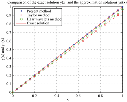
Figure 1. Image of analytical solution $y\left(x\right)$ and numerical solution $y_n(\; x\; )$

图1. 解析解 $y\left(x\right)$ 与数值解 $y_n\left(x\right)$ 的图像

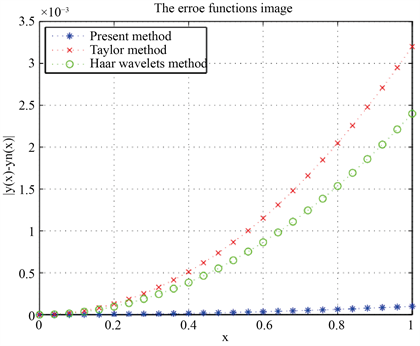
Figure 2. Image of error function $e_n$

图2. 误差函数 $e_n$ 图像

Table 1. Comparison results of analytical solution and numerical solution

表1. 解析解与数值解的对比结果

Table 2. Comparison of absolute error of different methods when N = 7

表2. 当N = 7，不同方法的绝对误差比较

可以发现贝塞尔多项式方法的结果比其他方法更接近精确解。随着多项式阶数的增加，贝塞尔多项式基函数法的精度逐渐提高。表2显示了当设置多项式的阶数为7时，泰勒法，Haar小波法和贝塞尔多项式方法的绝对误差的比较。可以发现，结果优于泰勒法和Haar小波法。泰勒方法和Haar小波方法的最小误差为 $O\left({10}^{-5}\right)$，但在多项式基函数的相同阶下，本文方法的有效误差已达到 $O\left({10}^{-\text{8}}\right)$。

5. 结论

第二类非线性Volterra积分方程的系统在物理、数学和工程中有着非常重要的作用。由于VIE的系统通常难以解析求解，因此需要得到近似解。因此，本文提出了基于贝塞尔多项式求解非线性Volterra积分方程的方法。此外，所提出的方法用于求解第二类非线性Volterra积分方程系统，表明该方法与其他方法相比具有较高的性能，并在数值算例中给出了数值结果。

基金项目

东华理工大学研究生创新基金(DHYC-202028)，江西省教育厅科学技术研究项目(GJJ200757)。

NOTES

^*通讯作者