(2 + 1)维非线性Ginzburg-Landau方程和广义Zakharov系统中的明暗光孤子解

Bright and Dark Soliton Solutions in the (2 + 1) Dimensional Nonlinear Ginzburg-Landau Equation and the Generalized Zakharov System

摘要: 研究(2 + 1)维非线性Ginzburg-Landau方程和广义Zakharov系统。运用待定系数的相关方法，探究(2 + 1)维非线性Ginzburg-Landau方程和广义Zakharov系统的明暗孤子解。最终获得了奇异波解和周期解等不同类型的精确解，并用Mathematica画出了相关的解的图像，并且本文所获得的孤子解是全新的。

Abstract: The paper studies the (2 + 1) dimensional nonlinear Ginzburg Landau equation and generalized Zakharov system. Using the relevant methods of undetermined coefficients, explore the bright dark soliton solutions of the (2 + 1) dimensional nonlinear Ginzburg-Landau equation and the general-ized Zakharov system. Finally, different types of exact solutions such as singular wave solutions and periodic solutions were obtained, and the relevant solutions were depicted using Mathematica. The soliton solutions obtained in this paper are brand new.

1. 简介

Ginzburg-Landau (GL)类型的方程是一种广泛应用于描述非线性介质中图案形成和时空混沌的通用模型，同时考虑了耗散和色散特性 [1] 。其中，cubic quintic (CQ)类型的GL模型最早由Petviashvili和Sergeev [2] 引入，用于描述二维情况下的稳定完全局部化的二维物体。此后，Thual和Fauve以及Deissler和Brand [3] 在GL类型的模型中研究了二维脉冲的特性。另外，Firth和Scroggie预测了在具有饱和吸收器的非线性二维GL方程中可能出现的局部化脉冲 [4] 。同样地，在Swift-Hohenberg类型的CQ方程中，也发现了二维脉冲的局部化现象 [5] 。在 [5] 中作者通过假设Swift-Hohenberg类型二维方程形式，发现了各种类型的稳定局域态，这些结果表明与一维的类孤子系统不同，因为一维的驼峰状解通常对横向扰动是不稳定的。不仅如此，该作者还使用了伪谱方法在边长为 $L^2=167r^2$ 的正方形盒子中进行了模拟，获得了相对明显的结果。此外，最近的研究表明，在具有CQ非线性的二维GL方程中，可以观察到稳定的局部化螺旋脉冲形态。

描述二维波导中电磁场局部振幅 $\omega \left(x,y,t\right)$ 演化的原型模型方程为：

$i{\omega }_t+\frac{1}{2}{\omega }_{xx}+\frac{1}{2}\left(\beta -iF\right){\omega }_{yy}+{\left|\omega \right|}^2\omega =i{\gamma }_0\omega ,$ (1)

在这里 $\beta ,F,{\gamma }_0$ 为常数。

描述线性增益和非线性饱和吸收相结合的最简单模型基于上述的CQ类型的GL方程。具体而言，相应修改后的二维方程的形式如下：

$i{\omega }_t+\frac{1}{2}{\omega }_{xx}+\frac{1}{2}\left(\beta -iF\right){\omega }_{yy}+\left(1-i{r}_1\right)\omega {\left|\omega \right|}^2+i{r}_2\omega {\left|\omega \right|}^4+i{\gamma }_0\omega =0.$ (2)

通过重新调整，可以将 ${\gamma }_0\equiv 1$ 和 $F\equiv 1$ 固定下来，那么方程(2)的最终形式为：

$i{\omega }_t+\frac{1}{2}{\omega }_{xx}+\frac{1}{2}\left(\beta -i\right){\omega }_{yy}+\left(1-i{r}_1\right)\omega {\left|\omega \right|}^2+i{r}_2\omega {\left|\omega \right|}^4+i\omega =0.$ (3)

广义Zakharov系统描述了离子化等离子体中Langmuir波的传播，该系统在物理学中有广泛的应用，具体方程形式如下 [6] [7] ：

$\{\begin{array}{l}i{A}_t+\alpha A_{xx}-{\rho }_{1}qA+{\rho }_{2}A{\left|A\right|}^2+{\rho }_{3}A{\left|A\right|}^4=0,\\ q_{tt}-m^2{q}_{xx}=\beta {\left({\left|A\right|}^2\right)}_{xx},\end{array}$ (4)

其中 $\alpha ,\beta ,{\rho }_1,{\rho }_2,{\rho }_3$ 和m是实数。参数m与离子声速成正比，未知函数 $q\left(x,t\right)$ 是离子密度相对于其平衡值的波动，而未知函数 $A\left(x,t\right)$ 是高度振荡电子场的缓变包络。早在2009年，Borhanifar等人利用Exp-function方法获得了广义Zakharov方程的广义孤立子解和周期解 [8] 。除此之外，在2011年，Al-Muhiameed等人也对其展开研究，利用一个改进的Jacobi elliptic function方法获得了该方程组的一系列精确行波解 [9] 。由此可知该方程的研究意义十分重大，有极大的研究价值。

本文将通过待定系数的方法 [10] - [21] 研究探讨(3)和(4)的明暗孤子解，并用Mathematica绘制出部分精确解的图像。

2. (2 + 1)维非线性Ginzburg-Landau方程

2.1. 明孤子解

为了得到(3)新的明孤子解，我们不妨假设(3)有如下形式的明孤子解

$\omega \left(x,y,t\right)=\mu \text{sech}\left(ax+by\right)\exp \left(i\lambda t\right),$ (5)

其中 $\lambda ,a,b,\mu$ 是(5)中的常数，将(5)代入(3)中，并收集 ${\cosh }^n,\left(n=0,2,4,6\right)$ 相应系数可得

$\{\begin{array}{l}\frac{a^2}{2}+\frac{b^2}{2}\left(\beta -i\right)+i-\lambda =0,\\ -a^2-b^2\left(i-\beta \right)+{\mu }^2\left(1-i{r}_1\right)=0,\\ i{\mu }^4{r}_2=0.\end{array}$ (6)

通过化简(6)即可得到如下结果

$\{\begin{array}{l}\lambda =\frac{a^2}{2}+\frac{b^2}{2}\left(\beta -i\right)+i,\\ \mu =\sqrt{\frac{a^2+b^2\left(\beta -i\right)}{1-i{r}_1}},\\ r_2=0.\end{array}$ (7)

最后可以得到

$\omega \left(x,y,t\right)=\sqrt{\frac{a^2+b^2\left(\beta -i\right)}{1-i{r}_1}}\text{sech}\left(ax+by\right)\text{exp}\left(it\left(\frac{a^2}{2}+\frac{b^2}{2}\left(\beta -i\right)+i\right)\right)$ (8)

在(8)中，取 $a=1,b=0,r_1=-2i,t=0$ 然后取其实部，可以获得图1。

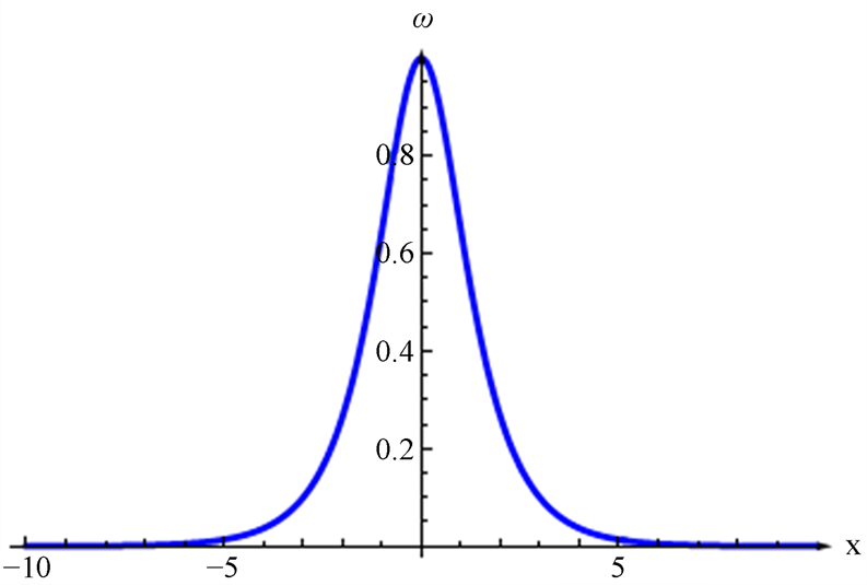
Figure 1. The real part plot of Equation (8)

图1. 公式(8)的实部图像

2.2. 奇异波解

为了得到(3)的奇异波解，我们不妨设(3)有如下形式的解

$\omega \left(x,y,t\right)=\mu \text{csch}\left(ax+by\right)\exp \left(i\lambda t\right).$ (9)

然后将(9)代入(3)，并收集 ${\cosh }^n,(n=0,2,4,6)$ 相应的系数，我们可以得到

$\{\begin{array}{l}-\frac{a^2}{2}-\frac{b^2}{2}\left(\beta -i\right)+i{\mu }^4{r}_2-{\mu }^2\left(1-i{r}_1\right)+i-\lambda =0,\\ \frac{a^2}{2}+\frac{b^2}{2}\left(\beta -i\right)+i-\lambda =0,\\ {\mu }^2\left(1-i{r}_1\right)-2i+2\lambda =0.\end{array}$ (10)

通过化简(10)我们可以得到

$\{\begin{array}{l}\lambda =\frac{a^2}{2}+\frac{b^2}{2}\left(\beta -i\right)+i,\\ \mu =\sqrt{\frac{-a^2-b^2\left(\beta -i\right)}{1-i{r}_1}},\\ r_2=0.\end{array}$ (11)

显然可以得到如下奇异波解

$\omega \left(x,y,t\right)=\sqrt{\frac{-a^2-b^2\left(\beta -i\right)}{1-i{r}_1}}\text{csch}\left(ax+by\right)\text{exp}\left(it\left(\frac{a^2}{2}+\frac{b^2}{2}\left(\beta -i\right)+i\right)\right)\text{.}$ (12)

取 $a=1,b=0,r_1=-2i,t=0$ 代入(12)，再取其实部可得图2。

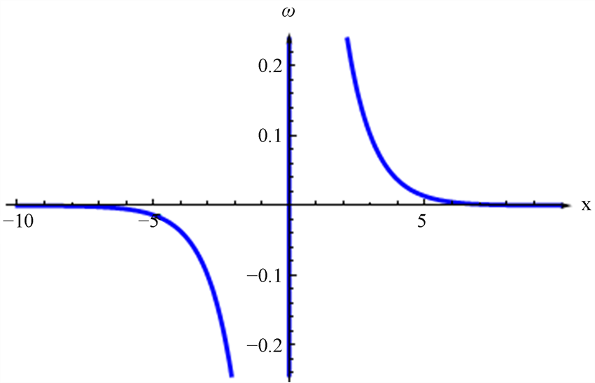
Figure 2. The real part plot of Equation (12)

图2. 公式(12)的实部图像

2.3. 周期波解

同样为了得到方程的周期波解，不妨设(3)有如下形式的周期波解

$\omega \left(x,y,t\right)=\mu \sec \left(ax+by\right)\exp \left(i\lambda t\right).$ (13)

然后将(13)代入(3)，并收集 ${\cos }^n\left(n=0,2,4,6\right)$ 相应的系数，我们可以得到

$\{\begin{array}{l}-\frac{a^2}{2}-\frac{b^2}{2}\left(\beta -i\right)+i+\lambda =0,\\ a^2+b^2\left(\beta -i\right)+{\mu }^2\left(1-i{r}_1\right)=0\\ i{\mu }^4{r}_2=0.\end{array}$ (14)

通过化简(14)我们可以得到

$\{\begin{array}{l}\lambda =-\frac{a^2}{2}-\frac{b^2}{2}\left(\beta -i\right)+i,\\ \mu =\sqrt{\frac{-a^2-b^2\left(\beta -i\right)}{1-i{r}_1}},\\ r_2=0.\end{array}$ (15)

显然可以得到如下周期波解

$\omega \left(x,y,t\right)=\sqrt{\frac{-a^2-b^2\left(\beta -i\right)}{1-i{r}_1}}\sec \left(ax+by\right)\exp \left(it\left(-\frac{a^2}{2}-\frac{b^2}{2}\left(\beta -i\right)+i\right)\right).$ (16)

取 $a=1,b=0,r_1=-2i,t=0$ 代入(16)，再取其实部可得图3。

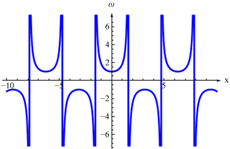
Figure 3. The real part plot of Equation (16)

图3. 公式(16)的实部图像

2.4. 暗孤子解

为了得到(3)的暗孤子解，不妨设(3)有如下形式的暗孤子解

$\omega \left(x,y,t\right)=\mu \tanh \left(ax+by\right)\exp \left(i\lambda t\right).$ (17)

将(17)代入(3)，并收集 ${\tanh }^n\left(n=1,3,5\right)$ 相应的系数，我们可以得到

$\{\begin{array}{l}\lambda =-a^2+b^2\left(i-\beta \right)+i,\\ \mu =\sqrt{\frac{a^2+b^2\left(\beta -i\right)}{i{r}_1-1}},\\ r_2=0.\end{array}$ (18)

显然可以得到如下暗孤子解

$\omega \left(x,y,t\right)=\sqrt{\frac{a^2+b^2\left(\beta -i\right)}{i{r}_1-1}}\tanh \left(ax+by\right)\exp \left(it\left(-a^2+b^2\left(i-\beta \right)+i\right)\right).$ (19)

取 $a=1,b=0,r_1=-2i,t=0$ 代入(19)，再取其实部可得图4。

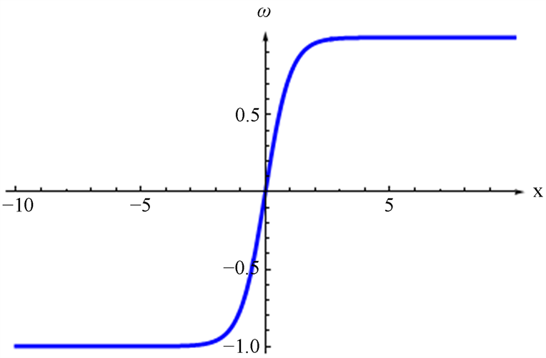
Figure 4. The real part plot of Equation (19)

图4. 公式(19)的实部图像

2.5. 周期波解

为了得到(3)的周期波解，不妨设(3)有如下形式的解

$\omega \left(x,y,t\right)=\mu \tan \left(ax+by\right)\exp \left(i\lambda t\right)$ (20)

将(20)代入(3)，并收集 ${\tan }^n\left(n=1,3,5\right)$ 相应的系数，我们可以得到

$\{\begin{array}{l}\lambda =a^2+b^2\left(\beta -i\right)+i,\\ \mu =\sqrt{\frac{-a^2-b^2\left(\beta -i\right)}{1-i{r}_1}},\\ r_2=0.\end{array}$ (21)

显然可以得到如下周期波解

$\omega \left(x,y,t\right)=\sqrt{\frac{-a^2-b^2\left(\beta -i\right)}{1-i{r}_1}}\tan \left(ax+by\right)\exp \left(it\left(a^2+b^2\left(\beta -i\right)+i\right)\right)$ (22)

取 $a=1,b=0,r_1=-2i,t=0$ 代入(22)，再取其实部可得图5。

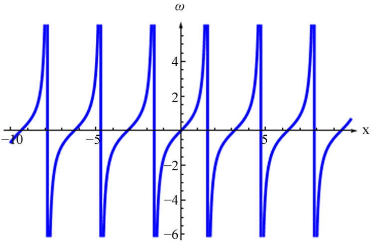
Figure 5. The real part plot of Equation (22)

图5. 公式(22)的实部图像

2.6. 其他解

为了确定指数解，我们假设指数解的结构为

$\omega \left(x,y,t\right)=\mu \exp \left(i\left(ax+by+\lambda t\right)\right).$ (23)

将(23)代入(3)可得

$\lambda =-\frac{1}{2}{a}^2-\frac{1}{2}{b}^2\left(\beta -i\right)+i{\mu }^4{r}_2+\mu \left(1-i{r}_1\right)+i,$ (24)

将(24)代入(23)可得

$\omega \left(x,y,t\right)=\mu \exp \left[i\left(t\left(-\frac{a^2}{2}-\frac{b^2}{2}\left(\beta -i\right)+i{\mu }^4{r}_2+{\mu }^2\left(1-i{r}_1\right)+i\right)+ax+by\right)\right]$ (25)

取 $a=1,b=0,\mu =1,t=0$ 代入(22)，再取其实部可得图6。

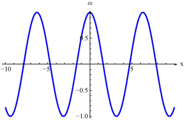
Figure 6. The real part plot of Equation (25)

图6. 公式(25)的实部图像

3. 非线性Zakharov系统

与前者运用相同的方式来研究非线性Zakharov系统需要进行一定的操作将其转化，具体操作如下：

$\{\begin{array}{l}i{A}_t+\alpha A_{xx}-{\rho }_{1}qA+{\rho }_{2}A{\left|A\right|}^2+{\rho }_{3}A{\left|A\right|}^4=0,\\ q_{tt}-m^2{q}_{xx}=\beta {\left({\left|A\right|}^2\right)}_{xx},\end{array}$ (26)

其中 $\alpha ,\beta \text{,}{\rho }_1,{\rho }_2,{\rho }_3$ 和m是实数。考虑该方程组解有如下形式

$A\left(x,t\right)=M\left(\xi \right)\exp \left[i\left(kx-wt\right)\right],q\left(x,t\right)=q\left(\xi \right),\xi =x-ct,$ (27)

其中 $k,w$ 和c是常数。接下来，不妨将(27)代入第二个式子，并进行二次积分，令积分常数为0可得

$q\left(\xi \right)=\frac{\beta M^2}{c^2-m^2}=\frac{\beta {\left|A\right|}^2}{c^2-m^2},$ (29)

将(29)代入(26)中的第一个式子，我们可以得到如下方程

$i{A}_t+\alpha A_{xx}+\left({\rho }_2-\frac{\beta {\rho }_1}{c^2-m^2}\right){\left|A\right|}^{2}A+{\rho }_3{\left|A\right|}^{4}A=0$ (30)

接下来我们就可以用 [10] - [18] 的方法来解决这一方程。

3.1. 明孤子解

为了得到(30)新的明孤子解，我们不妨假设(30)有如下形式的明孤子解

$A\left(x,t\right)=\mu \text{sech}\left(\xi \right)\exp \left[i\left(kx-wt\right)\right],\xi =x-ct$ (31)

将(31)代入(30)，并收集 ${\cosh }^n\left(n=0,2,4,6\right)$ 相应系数可得

$\{\begin{array}{l}\alpha -\alpha k^2+w=0,\\ {\mu }^2\left({\rho }_2-\frac{{\rho }_1\beta }{c^2-m^2}\right)-2\alpha =0,\\ {\rho }_3{\mu }^4=0,\\ c-2\alpha k=0.\end{array}$ (32)

通过化简(32)可得如下

$\{\begin{array}{l}w=\alpha \left(k^2-1\right),\\ \mu =\sqrt{\frac{2\alpha }{{\rho }_2-\frac{\beta {\rho }_1}{c^2-m^2}}}\\ {\rho }_3=0,\\ c=2\alpha k.\end{array},$ (33)

最后我们可以得到

$A\left(x,t\right)=\sqrt{\frac{2\alpha }{{\rho }_2-\frac{{\rho }_1\beta }{4{\alpha }^2{k}^2-m^2}}}\mathrm{sech}\left(x-2\alpha kt\right)\exp \left[i\left(kx-\alpha \left(k^2-1\right)t\right)\right]$ (34)

3.2. 奇异波解

同样地，不妨假设(30)有如下形式的奇异波解

$A\left(x,t\right)=\mu \text{csch}\left(\xi \right)\exp \left[i\left(kx-wt\right)\right],\xi =x-ct.$ (35)

将(35)代入(30)，与上个方程进行类似的操作即可得

$\{\begin{array}{l}\alpha -\alpha k^2+w=0\\ {\mu }^2\left({\rho }_2-\frac{{\rho }_1\beta }{c^2-m^2}\right)+2\alpha k^2-2w=0,\\ -\alpha -{\mu }^2\left({\rho }_2-\frac{{\rho }_1\beta }{c^2-m^2}\right)+{\rho }_3{\mu }^4-\alpha k^2+w=0,\\ c-2\alpha k=0.\end{array}$ (36)

通过化简(36)，我们可以得到

$\{\begin{array}{l}w=\alpha \left(k^2-1\right),\\ \mu =\sqrt{-\frac{2\alpha }{{\rho }_2-\frac{\beta {\rho }_1}{c^2-m^2}}},\\ {\rho }_3=0,\\ c=2\alpha k.\end{array}$ (37)

最终可以得到(30)奇异波解为

$A\left(x,t\right)=\sqrt{-\frac{2\alpha }{{\rho }_2-\frac{{\rho }_1\beta }{4{\alpha }^2{k}^2-m^2}}}\mathrm{csch}\left(x-2\alpha kt\right)\exp \left[i\left(kx-\alpha \left(k^2-1\right)t\right)\right].$ (38)

3.3. 周期波解

为了得到(30)的周期波，不妨设其周期波解的形式为

$A\left(x,t\right)=\mu \sec \left(\xi \right)\exp \left[i\left(kx-wt\right)\right],\xi =x-ct.$ (39)

将(39)代入(30)，与上个方程进行类似的操作即可得

$\{\begin{array}{l}-\alpha -\alpha k^2+w=0,\\ 2\alpha +{\mu }^2\left({\rho }_2-\frac{{\rho }_1\beta }{c^2-m^2}\right)=0,\\ {\rho }_3=0,\\ c=2\alpha k.\end{array}$ (40)

通过化简(40)，我们可以得到

$\{\begin{array}{l}w=\alpha \left(k^2+1\right),\\ \mu =\sqrt{-\frac{2\alpha }{{\rho }_2-\frac{\beta {\rho }_1}{c^2-m^2}}},\\ {\rho }_3=0,\\ c=2\alpha k.\end{array}$ (41)

最后可以得到周期波解的形式为

$A\left(x,t\right)=\sqrt{-\frac{2\alpha }{{\rho }_2-\frac{\beta {\rho }_1}{4{\alpha }^2{k}^2-m^2}}}\sec \left(x-2\alpha kt\right)\exp \left[i\left(kx-\alpha \left(k^2+1\right)t\right)\right]$ (42)

3.4. 暗孤子解

为了得到(30)的暗孤子解，不妨设其暗孤子解的形式为

$A\left(x,t\right)=\mu \tanh \left(\xi \right)\exp \left[i\left(kx-\omega t\right)\right],\xi =x-ct.$ (43)

将(43)代入(30)，与上个方程进行相同的操作

$\{\begin{array}{l}-2\alpha -\alpha k^2+w=0,\\ 2\alpha +{\mu }^2\left({\rho }_2-\frac{{\rho }_1\beta }{c^2-m^2}\right)=0,\\ {\rho }_3{\mu }^4=0,\\ c-2\alpha k=0.\end{array}$ (44)

通过化简(44)可以得到

$\{\begin{array}{l}\omega =\alpha \left(k^2+2\right),\\ \mu =\sqrt{-\frac{2\alpha }{{\rho }_2-\frac{\beta {\rho }_1}{c^2-m^2}}}\\ {\rho }_3=0,\\ c=2\alpha k.\end{array},$ (45)

最后我们可以得到

$A\left(x,t\right)=\sqrt{-\frac{2\alpha }{{\rho }_2-\frac{{\rho }_1\beta }{4{\alpha }^2{k}^2-m^2}}}\tanh \left(x-2\alpha kt\right)\exp \left[i\left(kx-\alpha \left(k^2+2\right)t\right)\right].$ (46)

3.5. 周期波解

为了得到(30)的周期波解，不妨设其周期波解的形式为

$A\left(x,t\right)=\mu \tan \left(\xi \right)\exp \left[i\left(kx-wt\right)\right],\xi =x-ct.$ (47)

将(47)代入(30)与上文进行类似的操作即可得

$\{\begin{array}{l}2\alpha -\alpha k^2+w=0,\\ 2\alpha +{\mu }^2\left({\rho }_2-\frac{{\rho }_1\beta }{c^2-m^2}\right)=0,\\ {\rho }_3=0,\\ c=2\alpha k.\end{array}$ (48)

通过化简(48)即可得到

$\{\begin{array}{l}w=\alpha \left(k^2-2\right),\\ \mu =\sqrt{-\frac{2\alpha }{{\rho }_2-\frac{\beta {\rho }_1}{c^2-m^2}}},\\ {\rho }_3=0,\\ c=2\alpha k.\end{array}$ (49)

最后我们可以得到方程的周期波解为

$A\left(x,t\right)=\sqrt{-\frac{2\alpha }{{\rho }_2-\frac{\beta {\rho }_1}{c^2-m^2}}}\tan \left(x-2\alpha kt\right)\exp \left[i\left(kx-\alpha \left(k^2-2\right)t\right)\right]$ (50)

3.6. 其他解

为了确定指数解，我们假设指数解的结构为

$A\left(x,t\right)=\mu \exp \left(i\left(x-wt\right)\right).$ (51)

将(51)代入(30)我们可以得到

$-\alpha +{\mu }^2\left(\rho -\frac{\beta {\rho }_1}{c^2-m^2}\right)+{\rho }_3{\mu }^4+w=0.$ (52)

通过化简(52)我们可以得到

$w=\alpha -{\mu }^2\left({\rho }_2-\frac{\beta {\rho }_1}{c^2-m^2}\right)-{\rho }_3{\mu }^4.$ (53)

最终获得该解为

$A\left(x,t\right)=\mu \exp \left[i\left(x-t\left(\alpha -{\mu }^2\left(-\frac{\beta {\rho }_1}{c^2-m^2}+{\rho }_2\right)-{\mu }^4{\rho }_3\right)\right)\right].$ (54)

4. 结论

利用该方法发现当 $r_2=0$ 时，方程(3)具有各种孤子解。类似地，当 ${\rho }_3=0$ 时，方程(4)具有各种精确解。通过计算，我们得到了方程(3)的各种精确解，如(8)，(12)，(16)，(19)，(22)和(25)。我们还得到了非线性广义Zakharov系统的孤子解为(34)，(38)，(42)，(46)，(50)和(54)。与其他论文中得到的相关孤子解相比，这种方法相对简单，并且需要较少的计算。所得到的解与本人所查阅文献中的这些解完全不同。但是本文所使用的待定系数法研究的解的形式是有限的，未来尝试使用分支方法以及扩展的辅助方程方法来研究这类方程的精确解。最后希望本文中得到的一些新解能为对非线性波感兴趣的研究人员提供一些帮助。