流固振动Laplace模型的有限元局部并行方案

Local and Parallel Finite Element Algorithms to Solve Laplace Model for Fluid-Solid Vibrations

摘要: 本文研究流固振动Laplace模型的局部和并行有限元算法，首先给出流固振动Laplace模型的局部先验误差估计，然后建立局部和并行有限元方案，并给出局部方案的误差分析，最后给出数值算例验证方案的有效性。

Abstract: In this paper, for the Laplace model for fluid-solid vibrations we establish the local finite element discretization scheme. We give the local a priori error estimate and the error analysis of the proposed scheme. We also provide the numerical experiment to show the efficiency of our scheme.

1. 引言

局部先验估计是有限元方法的基本研究内容，基于局部先验估计的局部并行算法是求解偏微分方程的高效数值方法之一。2000年许进超和周爱辉结合局部亏量校正技巧的二网格离散方法，提出了有限元局部和并行算法，并用于求解二阶非对称边值问题(参见文献 [1] )。之后，许多学者发展该方法，将之成功用于Stokes方程(参见 [2] [3] )，量子特征值问题(参见 [4] )，对流扩散方程(参见 [5] )，定常不可压缩流问题(参见 [6] )，二阶椭圆特征值问题(参见 [7] [8] )，Steklov特征值问题(参见 [9] [10] )和传输特征值问题(参见 [11] )等。

流固振动Laplace模型问题来源于浸没在不可压缩流体中的一束平行管的振动，在核工程中具有相当重要的意义(参见文献 [12] [13] [14] )，其数值方法近年受到诸多学者的关注，例如Armentano等研究了该问题的hp协调有限元法及自适应算法，并给出了先验误差估计和后验误差估计(参见 [15] )，张宇等用非协调有限元方法研究了流固振动特征值的可保证下界(参见 [16] )。本文研究流固振动Laplace模型的局部先验误差估计和有限元局部计算方法，首先给出该问题的局部先验估计，基于局部先验估计建立协调有限元局部计算方案，接着对方案进行误差分析，最后给出数值实验展示局部和并行方案的效率。

关于有限元法和谱逼近的基本理论参见文献 [17] [18]。本文中字母C表示与网格尺寸无关的常数，它在不同的地方所表示的值可能不同。为方便起见用符号 $a\lesssim b$ 表示 $a\le Cb$。

2. 预备知识

考虑下述流固振动Laplace模型(详见 [12] [14] [19] )：求 $\omega >0$ (振动频率)， $u\ne 0$ (流体压力)使得

$\begin{array}{r}\hfill \{\begin{array}{l}\Delta u=0在\Omega 中,\\ \frac{\partial u}{\partial n}=0在{\Gamma }_0上,\\ \frac{\partial u}{\partial n}=\frac{\rho {\omega }^2}{\mu -m{\omega }^2}\left({\displaystyle {\int }_{{\Gamma }_i}un\text{d}s}\right)\cdot n在{\text{Γ}}_i上,i=1,2,\cdots ,K,\end{array}\end{array}$ (2.1)

这里 $\Omega \subset {ℝ}^2$ 是由流体占据的有界多边形区域， ${\Gamma }_0$ 表示 $\Omega$ 的外边界， ${\Gamma }_i\left(i=1,\cdots ,K\right)$ 表示每个管与流体间的交界面，管的硬度为 $\mu$，质量为m，流体视为完全不可压缩且密度为 $\rho$， $n={\left(n_1,n_2\right)}^{\text{T}}$ 是 $\Omega$ 边界上的单位外法向量。记 $\Gamma ={\Gamma }_0\cup {\Gamma }_1\cup \cdots \cup {\Gamma }_K$ (参见图1)。

令 $H^t\left(\Omega \right)$ 表示 $\Omega$ 上通常t阶Sobolev空间，其上范数和半范数分别为 ${\Vert \cdot \Vert }_{t,\Omega }$ 和 ${\left|\cdot \right|}_{t,\Omega }$， $H^0\left(\Omega \right)=L_2\left(\Omega \right)$， $H^0\left(\Gamma \right)=L_2\left(\Gamma \right)$ 装备范数 ${\Vert \cdot \Vert }_{0,\Gamma }$。令 $V:=H^1\left(\Omega \right)/ℝ$，其上范数为 ${\left|\cdot \right|}_{1,\Omega }$。记 $\lambda :=\rho {\omega }^2/\left(\mu -m{\omega }^2\right)$。(2.1)的弱形式为：求 $\lambda \in ℝ$， $u\in V$ 满足

$\{\begin{array}{l}a\left(u,v\right)=\lambda b\left(u,v\right)\forall v\in V,\hfill \\ b\left(u,u\right)=1,\hfill \end{array}$ (2.2)

其中

$\begin{array}{l}a\left(u,v\right)={\displaystyle {\int }_{\Omega }\nabla u\cdot \nabla v},\\ b\left(u,v\right)=\underset{i=1}{\overset{K}{{\displaystyle \sum }}}\left({\displaystyle {\int }_{{\Gamma }_i}un}\right)\cdot \left({\displaystyle {\int }_{{\Gamma }_i}vn}\right),{\left|u\right|}_b=b{\left(u,u\right)}^{\frac{1}{2}}\text{.}\end{array}$

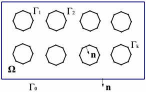
Figure 1. Schematic diagram of 2D area model

图1. 二维区域模型示意图

显然 $a\left(\cdot ,\cdot \right)$ 是 $V\times V$ 上连续、对称、椭圆的双线性形式， $b\left(\cdot ,\cdot \right)$ 是 $V\times V$ 上非负、连续、对称的双线性形式。由文献 [19] 可知，(2.2)的解是由2K个特征对 $\left({\lambda }_j,u_j\right)$ 给出的序列，其中特征值 ${\lambda }_j$ 均为正，假设特征值按递增排序： $0<{\lambda }_1\le \cdots \le {\lambda }_{2K}$。相应于特征值 ${\lambda }_j$ 的特征函数 $u_j\in V$ 使得 $\left\{u_1,\cdots ,u_{2K}\right\}$ 是一个线性无关集。

令 ${\pi }_h\left(\Omega \right)$ 是 $\Omega$ 的一族三角形剖分， $h\left(x\right)$ 是点x所在单元T的直径， $h_{\Omega }={\max }_{x\in \Omega }h\left(x\right)$ 是剖分 ${\pi }_h\left(\Omega \right)$ 的直径。令 ${\epsilon }_h\left({\Gamma }_i\right)=\left\{e\right\}$ 表示 ${\pi }_h\left(\Omega \right)$ 中位于边界 ${\Gamma }_i$ 上的边组成的集合， ${\epsilon }_h\left(\Gamma \right)={\epsilon }_h\left({\Gamma }_1\right)\cup {\epsilon }_h\left({\Gamma }_2\right)\cup \cdots \cup {\epsilon }_h\left({\Gamma }_K\right)$。令 $S_h\left(\Omega \right)\subset C\left(\bar{\Omega }\right)$ 是定义在 ${\pi }_h\left(\Omega \right)$ 上的分片m次多项式空间， $V_h\left(\Omega \right)=S_h\left(\Omega \right)/ℝ$。

相应于(2.2)的离散特征值问题为：求 ${\lambda }_h\in ℝ$ 和 $u_h\in V_h\left(\Omega \right)$ 满足

$\{\begin{array}{l}a\left(u_h,v_h\right)={\lambda }_{h}b\left(u_h,v_h\right)\forall v_h\in V_h\left(\Omega \right),\hfill \\ b\left(u_h,u_h\right)=1.\hfill \end{array}$ (2.3)

由文献 [19] 可知，离散问题(2.3)具有2K个正的特征值，假设特征值按递增排序： $0<{\lambda }_{1,h}\le \cdots \le {\lambda }_{2K,h}$，相应于特征值 ${\lambda }_{j,h}$ 的特征函数 $u_{j,h}\in V_h\left(\Omega \right)$ 使得 $\left\{u_{1,h},\cdots ,u_{2K,h}\right\}$ 是一个线性无关集。

相应于(2.2)的源问题与相应于(2.3)的近似源问题分别如下：

求 $w\in V$，使得

$a\left(w,v\right)=b\left(f,v\right),\forall v\in V;$ (2.4)

求 $w_h\in V_h\left(\Omega \right)$，使得

$\begin{array}{r}\hfill a\left(w_h,v\right)=b\left(f,v\right),\forall v\in V_h\left(\Omega \right)\text{.}\end{array}$ (2.5)

记

$\tilde{f}=\left({\displaystyle {\int }_{{\Gamma }_i}fn}\right)\cdot n\text{on}{\Gamma }_i,i=1,\cdots ,K;\tilde{f}=0\text{on}{\Gamma }_0,$

经简单计算有

${\left|f\right|}_b\le C{\Vert f\Vert }_{0,\Gamma },$ (2.6)

于是，对 $f\in L^2\left(\Gamma \right)$ 有

$\begin{array}{c}{\displaystyle \underset{\Gamma }{\int }{\tilde{f}}^2\text{d}s}={\displaystyle \underset{i=1}{\overset{K}{\sum }}{\displaystyle \underset{{\Gamma }_i}{\int }\left({\displaystyle {\int }_{{\Gamma }_i}fn}\right)\cdot n\left({\displaystyle {\int }_{{\Gamma }_i}fn}\right)\cdot n\text{d}s}}\\ \le C{\displaystyle \underset{i=1}{\overset{K}{\sum }}\left({\displaystyle {\int }_{{\Gamma }_i}fn}\right)\cdot \left({\displaystyle {\int }_{{\Gamma }_i}fn}\right)\text{d}s}\le C{\left|f\right|}_b^2\lesssim {\Vert f\Vert }_{0,\Gamma }^2,\end{array}$

这表明 $\tilde{f}\in L^2\left(\Gamma \right)$。因此，由Neumann问题先验估计(参见文献 [20]，或文献 [21] 命题4.4)可知，(2.4)的解 $w\in H^{1+\frac{r}{2}}\left(\Omega \right)$ 且满足

${\Vert w\Vert }_{H^{1+\frac{r}{2}}\left(\Omega \right)/ℝ}\lesssim {\Vert \tilde{f}\Vert }_{0,\Gamma }\lesssim {\left|f\right|}_b\lesssim {\Vert f\Vert }_{0,\Gamma }\lesssim {\left|f\right|}_{1,\Omega },$ (2.7)

其中 $r<\frac{\pi }{\theta }$， $\theta$ 为区域 $\Omega$ 的最大凹角。于是，对所有 $r<\frac{\pi }{\theta }$，(2.2)的特征函数 $u\in H^{1+\frac{r}{2}}\left(\Omega \right)$。注意，对于具有至少一个交界面 ${\Gamma }_i$ 的多角形区域 $\Omega$，必有 $\theta >\pi$，因此 $\frac{1}{2}<\frac{\pi }{\theta }<1$。

根据Lax-Milgram定理可知，(2.4)和(2.5)分别存在唯一解，于是可定义解算子 $T,T_h:V\to V$ ：

$\begin{array}{c}\{\begin{array}{l}f\in V\mapsto Tf\in V,\\ a\left(Tf,v\right)=b\left(f,v\right)\forall v\in V;\end{array}\end{array}$

$\begin{array}{r}\hfill \{\begin{array}{l}f\in V\mapsto T_{h}f\in V_h\left(\Omega \right)\subset V,\hfill \\ a\left(T_{h}f,v_h\right)=b\left(f,v_h\right)\forall v_h\in V_h\left(\Omega \right).\hfill \end{array}\end{array}$

于是，(2.2)和(2.3)分别具有下述等价算子形式：

$Tu=\mu u,$ (2.8)

$T_h{u}_h={\mu }_h{u}_h,$ (2.9)

其中 $\mu =\frac{1}{\lambda },{\mu }_h=\frac{1}{{\lambda }_h}$。

由(2.7)可知 ${\Vert Tf\Vert }_{H^{1+\frac{r}{2}}\left(\Omega \right)/ℝ}\lesssim {\Vert f\Vert }_{0,\Gamma }\lesssim {\left|f\right|}_{1,\Omega }$，即算子T有界。

由(2.6)有

${\left|T_{h}f\right|}_{1,\Omega }^2=a\left(T_{h}f,T_{h}f\right)=b\left(f,T_{h}f\right)\lesssim {\left|f\right|}_b{\left|T_{h}f\right|}_b\lesssim {\Vert f\Vert }_{0,\Gamma }{\left|T_{h}f\right|}_{1,\Omega },$

从而 ${\left|T_{h}f\right|}_{1,\Omega }\lesssim {\Vert f\Vert }_{0,\Gamma }\lesssim {\left|f\right|}_{1,\Omega }$，即 $T_h$ 也是有界算子。

令 $M\left(\lambda \right)$ 表示所有相应于特征值 $\lambda$ 的特征函数张成的空间。

定义Ritz投影 $P_h:V\mapsto V_h\left(\Omega \right)$ 满足

$\begin{array}{r}\hfill a\left(w-P_{h}w,v\right)=0\forall v\in V_h\left(\Omega \right).\end{array}$

显然有

$\begin{array}{r}\hfill {\left|P_{h}w\right|}_{1,\Omega }\le {\left|w\right|}_{1,\Omega }\forall w\in V\text{.}\end{array}$

容易证明 $T_h=P_{h}T$。

利用Cea引理和Aubin-Nische技巧可得以下结论。

引理2.1 令w和 $w_h$ 分别是(2.4)和(2.5)的解，如果 $w\in H^{m+\sigma }\left(\Omega \right)\left(0<\sigma \le 1\right)$，则

${\left|w-P_{h}w\right|}_{1,\Omega }\le C{h}^{m+\sigma -1}{\Vert w\Vert }_{m+\sigma ,\Omega },$ (2.10)

${\Vert w-P_{h}w\Vert }_{0,\Omega }\le C{h}^{\frac{r}{2}}{\left|w-P_{h}w\right|}_{1,\Omega },$ (2.11)

${\Vert w-P_{h}w\Vert }_{0,\Gamma }\le C{h}^{\frac{r}{2}}{\left|w-P_{h}w\right|}_{1,\Omega }.$ (2.12)

引理2.2 算子T是紧的，且当 $h\to 0$ 时

${\Vert T_h-T\Vert }_{0,\Gamma }\to 0.$

证明：可记 $w=Tf$， $w_h=T_{h}f$，注意到 $T_h=P_{h}T$，由(2.10)，(2.11)及(2.7)有

$\begin{array}{c}{\Vert T_h-T\Vert }_{0,\Gamma }=\underset{0\ne f\in L^2\left(\Gamma \right)}{\sup }\frac{{\Vert T_{h}f-Tf\Vert }_{0,\Gamma }}{{\Vert f\Vert }_{0,\Gamma }}\le \underset{0\ne f\in L^2\left(\Gamma \right)}{\sup }\frac{C{h}^{\frac{r}{2}}{\left|T_{h}f-Tf\right|}_{1,\Omega }}{{\Vert f\Vert }_{0,\Gamma }}\\ \le \underset{0\ne f\in L^2\left(\Gamma \right)}{\sup }\frac{C{h}^r{\Vert Tf\Vert }_{1+\frac{r}{2}}}{{\Vert f\Vert }_{0,\Gamma }}\le C{h}^r\to 0\left(h\to 0\right).\end{array}$

证毕。

由谱逼近理论(参见文献 [17] 和文献 [15] 中命题3.1)，有以下引理。

引理2.3 设 $M\left(\lambda \right)\subset H^{m+\sigma }\left(\Omega \right)\left(0<\sigma \le 1\right)$，对所有的 $r<\frac{\pi }{\theta }$，存在正常数C和 $\kappa$ 使得当 $h<\kappa$ 时有

${\left|u_j-u_{j,h}\right|}_{1,\Omega }\lesssim h^{m+\sigma -1},$ (2.13)

${\left|u_j-u_{j,h}\right|}_b\lesssim h^{\frac{r}{2}}{\left|u_j-u_{j,h}\right|}_{1,\Omega },$ (2.14)

${\Vert u_j-u_{j,h}\Vert }_{0,\Gamma }\lesssim h^{\frac{r}{2}}{\left|u_j-u_{j,h}\right|}_{1,\Omega },$ (2.15)

$\left|{\lambda }_j-{\lambda }_{j,h}\right|\lesssim {\left|u_j-u_{j,h}\right|}_{1,\Omega }^2.$ (2.16)

引理2.4 设 $\left(\lambda ,u\right)$ 是(2.2)的特征对，则对任意 $v\in V$， $b\left(v,v\right)\ne 0$，有

$\begin{array}{r}\hfill \frac{a\left(v,v\right)}{b\left(v,v\right)}-\lambda =\frac{{\left|v-u\right|}_{1,\Omega }}{b\left(v,v\right)}-\lambda \frac{b\left(v-u,v-u\right)}{b\left(v,v\right)}\text{.}\end{array}$

证明：参见文献 [17] 引理9.1。

3. 局部先验误差估计

对于 $D\subset G\subset \Omega$，我们用符号 $D\subset \subset G$ 表示 $\text{dist}\left(\partial D\backslash \Gamma ,\partial G\backslash \Gamma \right)>0$。给定 $G\subset \Omega$，定义 ${\pi }_h\left(G\right)$ 和 $V_h\left(G\right)$ 分别表示 ${\pi }_h\left(\Omega \right)$ 和 $V_h\left(\Omega \right)$ 在G上的限制。记 $suppv=\overline{\left\{x:v\left(x\right)\ne 0\right\}}$， $V_h^0\left(G\right)=\left\{v\in V_h\left(\Omega \right):{v|}_{\partial G\backslash \Gamma }=0\right\}$ 和 $V_0^h\left(G\right)=\left\{v\in V_h\left(\Omega \right):\left(suppv\backslash \Gamma \right)\subset \subset G\right\}$。

令 ${\Omega }_0\subset \Omega$，假设本文的网格和有限元空间满足以下条件(参见文献 [1] )：

(A0) 存在 $\gamma \ge 1$，使得

$h_{\Omega }^{\gamma }\lesssim h\left(x\right),\forall x\in \Omega \text{.}$

(A1) 对 $w\in H^{1+s}\left(\Omega \right)$，存在 $m\ge 1$，使得

$\underset{v\in V_h\left(\Omega \right)}{\inf }\left({\Vert h^{-1}\left(w-v\right)\Vert }_{0,\Omega }+{\left|w-v\right|}_{1,\Omega }\right)\lesssim h^s{\Vert w\Vert }_{1+s,\Omega }0\le s\le m\text{.}$

(A2) 对任意 $v\in V_h\left({\Omega }_0\right)$，有

${\left|v\right|}_{1,{\Omega }_0}\lesssim {\Vert h^{-1}\left(x\right)v\Vert }_{0,{\Omega }_0}\text{.}$

(A3) 对 $G\subset {\Omega }_0$，令 $\omega \in C^{\infty }\left(\bar{\Omega }\right)$ 且 $\left(supp\omega \backslash \Gamma \right)\subset \subset G$。对任意 $w\in V_h\left(G\right)$，存在 $v\in V_0^h\left(G\right)$ 使得

${\left|h^{-1}\left(x\right)\left(\omega w-v\right)\right|}_{1,G}\lesssim {\left|w\right|}_{1,G}\text{.}$

对 $G\subset \Omega$，考虑下述混合边值问题：

$\begin{array}{l}\Delta \psi =g\text{in}G,\\ \psi =0\text{on}\partial G\backslash \Gamma ,\\ \frac{\partial \psi }{\partial n}=0\text{on}\partial G\cap \Gamma \text{.}\end{array}$ (3.1)

(3.1)的弱形式为：求 ${\psi }_g\in H_{\Gamma }^1\left(G\right)=\left\{v\in H^1\left(G\right):{v|}_{\partial G\backslash \Gamma }=0\right\}$ 使得

$\begin{array}{r}\hfill a\left(v,{\psi }_g\right)=\left(g,v\right),\forall v\in H_{\Gamma }^1\left(G\right),\end{array}$

其中 $\left(f,v\right)={\displaystyle {\int }_{\Omega }fv\text{d}x}$。

对(3.1)，我们作下述假设。

$R\left(G\right)$.对任意 $g\in L_2\left(G\right)$，存在 ${\psi }_g\in H_{\Gamma }^{1+r}\left(G\right)$ 满足

$a\left(v,{\psi }_g\right)=\left(g,v\right),\forall v\in H_{\Gamma }^1(\; G\; )$

且

${\Vert {\psi }_g\Vert }_{1+r,G}\le C{\Vert g\Vert }_{0,G}$.

由文献 [1] [10]，我们有下述引理。

引理3.1 令 $D\subset \subset {\Omega }_0\subset \Omega$， $\omega \in C^{\infty }\left(\bar{\Omega }\right)$， $\left(supp\omega \backslash \Gamma \right)\subset \subset {\Omega }_0$，则有

$a\left(\omega w,\omega w\right)\lesssim a\left(w,{\omega }^{2}w\right)+{\Vert w\Vert }_{0,{\Omega }_0}^2,\forall w\in H^1\left(\Omega \right)\text{.}$

引理3.2 设(A0)，(A2)及(A3)成立，且 $D\subset \subset {\Omega }_0$。若 $\mathcal{F}\in H^{-1}\left(\Omega \right)$ 和 $w\in V_h\left({\Omega }_0\right)$ 满足

$\begin{array}{r}\hfill a\left(w,v\right)=\mathcal{F}\left(v\right)\forall v\in V_0^h\left({\Omega }_0\right),\end{array}$

则有

${\left|w\right|}_{1,D}\lesssim {\Vert w\Vert }_{0,{\Omega }_0}+{\Vert \mathcal{F}\Vert }_{-1,{\Omega }_0}.$

定理3.1 设 $w\in V$， $D\subset \subset {\Omega }_0$，(A0)，(A1)，(A2)和(A3)成立，则

$\begin{array}{r}\hfill {\left|P_{h}w\right|}_{1,D}\lesssim {\left|w\right|}_{1,{\Omega }_0}+{\Vert P_{h}w\Vert }_{0,{\Omega }_0}\text{.}\end{array}$

证明：定义Ritz投影 $P_h^{{\Omega }_0}:V\left({\Omega }_0\right)\mapsto V_h\left({\Omega }_0\right)$ 满足

$a\left(w-P_h^{{\Omega }_0}w,v\right)=0,\forall v\in V_h\left({\Omega }_0\right)\text{.}$

取 $D_1\subset \Omega$ 满足 $D\subset \subset D_1\subset \subset {\Omega }_0$，并取 $\omega \in C^{\infty }\left(\bar{\Omega }\right)$ 使得在 $\overline{D_1}$ 上 $\omega \equiv 1$ 且 $\left(supp\omega \backslash \Gamma \right)\subset \subset {\Omega }_0$。令 $\tilde{w}=\omega w$，则对任意 $v\in V_0^h\left(D_1\right)$ 有

$a\left(P_h^{{\Omega }_0}\tilde{w}-P_{h}w,v\right)=a\left(P_h^{{\Omega }_0}\left(\omega w\right)-\omega w,v\right)-a\left(P_{h}w-\omega w,v\right)=0.$

于是，由引理3.2有

${\left|P_h^{{\Omega }_0}\tilde{w}-P_{h}w\right|}_{1,D}\lesssim {\Vert P_h^{{\Omega }_0}\tilde{w}-P_{h}w\Vert }_{0,D_1}\text{.}$

因此，利用商空间等价模定理推出

$\begin{array}{c}{\left|P_{h}w\right|}_{1,D}\lesssim {\left|P_h^{{\Omega }_0}\tilde{w}\right|}_{1,D}+{\left|P_h^{{\Omega }_0}\tilde{w}-P_{h}w\right|}_{1,D}\\ \lesssim {\left|P_h^{{\Omega }_0}\tilde{w}\right|}_{1,D}+{\Vert P_h^{{\Omega }_0}\tilde{w}-P_{h}w\Vert }_{0,D_1}\\ \lesssim {\left|P_h^{{\Omega }_0}\tilde{w}\right|}_{1,D_1}+{\Vert P_{h}w\Vert }_{0,D_1}+{\Vert P_h^{{\Omega }_0}\tilde{w}\Vert }_{0,D_1}\\ \lesssim {\left|P_h^{{\Omega }_0}\tilde{w}\right|}_{1,D_1}+{\Vert P_{h}w\Vert }_{0,D_1}+{\Vert P_h^{{\Omega }_0}\tilde{w}\Vert }_{1,D_1}\\ \lesssim {\left|P_h^{{\Omega }_0}\tilde{w}\right|}_{1,D_1}+{\Vert P_{h}w\Vert }_{0,D_1}+{\left|P_h^{{\Omega }_0}\tilde{w}\right|}_{1,D_1}\\ \lesssim {\left|\tilde{w}\right|}_{1,{\Omega }_0}+{\Vert P_{h}w\Vert }_{0,D_1}\lesssim {\left|w\right|}_{1,{\Omega }_0}+{\Vert P_{h}w\Vert }_{0,{\Omega }_0}.\end{array}$

证毕。

定理3.2 设 $w\in V$， $D\subset \subset {\Omega }_0$，(A0)，(A1)，(A2)和(A3)成立，则

$\begin{array}{r}\hfill {\left|w-P_{h}w\right|}_{1,D}\lesssim \underset{v\in V_h\left(\Omega \right)}{\inf }{\left|w-v\right|}_{1,{\Omega }_0}+{\Vert w-P_{h}w\Vert }_{0,\Omega }\text{.}\end{array}$

证明：对任意 $v\in V_h\left(\Omega \right)$，由定理3.1有

$\begin{array}{r}\hfill {\left|P_{h}w-v\right|}_{1,D}={\left|P_{h}w-P_{h}v\right|}_{1,D}\lesssim {\left|w-v\right|}_{1,{\Omega }_0}+{\Vert P_{h}w-v\Vert }_{0,{\Omega }_0},\end{array}$

于是

$\begin{array}{c}{\left|w-P_{h}w\right|}_{1,D}\lesssim {\left|w-v\right|}_{1,D}+{\left|v-P_{h}w\right|}_{1,D}\\ \lesssim {\left|w-v\right|}_{1,{\Omega }_0}+{\Vert v-P_{h}w\Vert }_{0,{\Omega }_0}\\ \lesssim {\left|w-v\right|}_{1,{\Omega }_0}+{\Vert v-w\Vert }_{0,{\Omega }_0}+{\Vert w-P_{h}w\Vert }_{0,{\Omega }_0}\\ \lesssim {\left|w-v\right|}_{1,{\Omega }_0}+{\Vert v-w\Vert }_{1,{\Omega }_0}+{\Vert w-P_{h}w\Vert }_{0,{\Omega }_0}\\ \lesssim {\left|w-v\right|}_{1,{\Omega }_0}+{\Vert w-P_{h}w\Vert }_{0,{\Omega }_0},\end{array}$

因此

$\begin{array}{r}\hfill {\left|w-P_{h}w\right|}_{1,D}\lesssim \underset{v\in V_h\left(\Omega \right)}{\inf }{\left|w-v\right|}_{1,{\Omega }_0}+{\Vert w-P_{h}w\Vert }_{0,\Omega }\text{.}\end{array}$

证毕。

定理3.3 在定理3.2的假设下，令 $\left({\lambda }_h,u_h\right)$ 是(2.3)的第j个特征对， $\lambda$ 是(2.2)的第j个特征值，则存在 $u\in M\left(\lambda \right)$ 使得下列误差估计成立

${\left|u-u_h\right|}_{1,D}\lesssim \underset{v\in V_h\left(\Omega \right)}{\inf }{\left|u-v\right|}_{1,{\Omega }_0}+{\Vert u-P_{h}u\Vert }_{0,\Omega }+{\Vert \lambda u-{\lambda }_h{u}_h\Vert }_{0,\Gamma }\text{.}$

证明：由(2.8)和(2.9)可推出

$\begin{array}{c}u-u_h=\lambda Tu-{\lambda }_h{T}_h{u}_h\\ =\lambda Tu-\lambda T_{h}u+\lambda T_{h}u-{\lambda }_h{T}_h{u}_h\\ =u-\lambda P_{h}Tu+T_h\left(\lambda u-{\lambda }_h{u}_h\right)\\ =u-P_{h}u+T_h\left(\lambda u-{\lambda }_h{u}_h\right),\end{array}$

因此

$\begin{array}{c}{\left|u-u_h\right|}_{1,D}\lesssim {\left|u-P_{h}u\right|}_{1,D}+{\left|T_h\left(\lambda u-{\lambda }_h{u}_h\right)\right|}_{1,D}\\ \lesssim {\left|u-P_{h}u\right|}_{1,D}+{\Vert \lambda u-{\lambda }_h{u}_h\Vert }_{0,\Gamma }\text{.}\end{array}$

利用定理3.2可得

$\begin{array}{c}{\left|u-u_h\right|}_{1,D}\lesssim {\left|u-P_{h}u\right|}_{1,D}+{\Vert \lambda u-{\lambda }_h{u}_h\Vert }_{0,\Gamma }\\ \lesssim \underset{v\in V_h\left(\Omega \right)}{\inf }{\left|u-v\right|}_{1,{\Omega }_0}+{\Vert u-P_{h}u\Vert }_{0,\Omega }+{\Vert \lambda u-{\lambda }_h{u}_h\Vert }_{0,\Gamma }\text{.}\end{array}$

证毕。

4. 局部和并行有限元方案

设 ${\pi }_H\left(\Omega \right)$ 是 $\Omega$ 的一个形正规网格，网格直径 $H\in \left(0,1\right)$， $D\subset \Omega$ 是包含奇点的一个子域，并设 ${\Omega }_0$ 是一个比D稍大的子域(即 $D\subset \subset {\Omega }_0$ )。令 ${\pi }_k\left(\Omega \right)$ 是在 ${\pi }_H\left(\Omega \right)$ 基础上加密得到的全局中网格， ${\pi }_h\left({\Omega }_0\right)$ 是在 ${\pi }_k\left(\Omega \right)$ 基础上通过局部加密得到的局部细网格，网格直径满足 $h\ll k\ll H$。

方案1 (局部计算方案)：

步骤1在全局粗网格 ${\pi }_H\left(\Omega \right)$ 上解(2.3)：求 ${\lambda }_H\in ℝ$， $u_H\in V_H\left(\Omega \right)$ 使得 ${\left|u_H\right|}_{1,\Omega }=1$ 且

$a\left(u_H,v\right)={\lambda }_{H}b\left(u_H,v\right),\forall v\in V_H\left(\Omega \right)\text{.}$

步骤2在全局中网格 ${\pi }_k\left(\Omega \right)$ 上解线性边值问题：求 $u^k\in V_k\left(\Omega \right)$ 使得

$\begin{array}{r}\hfill a\left(u^k,v\right)={\lambda }_{H}b\left(u_H,v\right),\forall v\in V_k\left(\Omega \right)\text{.}\end{array}$

步骤3在局部加密细网格 ${\pi }_h\left({\Omega }_0\right)$ 上解线性边值问题：求 $e^h\in V_h^0\left({\Omega }_0\right)$ 使得

$\begin{array}{r}\hfill a\left(e^h,v\right)={\lambda }_{H}b\left(u_H,v\right)-a\left(u^k,v\right),\forall v\in V_h^0\left({\Omega }_0\right)\text{.}\end{array}$

步骤4令

$u^{k,h}=\{\begin{array}{l}{u}^k+e^h\text{on}{\bar{\Omega }}_0\\ u^k\text{in}\Omega \backslash {\bar{\Omega }}_0\end{array}$

计算Rayleigh商

${\lambda }^{k,h}=\frac{a\left(u^{k,h},u^{k,h}\right)}{b\left(u^{k,h},u^{k,h}\right)}.$

定理4.1 设 $u^{k,h}$ 是由方案1计算所得，且 $R\left({\Omega }_0\right)$ 和A(0)~A(3)成立。若 $M\left(\lambda \right)\subset H^1\left(\Omega \right)\cap H^{m+\sigma }\left(\Omega \right)\cap H^{m+1}\left(\Omega \backslash \bar{D}\right)$ ( $1<m+\sigma$ 且 $0\le \sigma <1$ )，则

$\begin{array}{r}\hfill {\left|u-u^{k,h}\right|}_{1,\Omega }\lesssim h^{m+\sigma -1}+k^m+H^{m+\sigma -1+\frac{r}{2}},\end{array}$ (4.1)

$\begin{array}{r}\hfill \left|\lambda -{\lambda }^{k,h}\right|\lesssim h^{2m+2\sigma -2}+k^{2m}+H^{2m+2\sigma -2+r}\text{.}\end{array}$ (4.2)

证明：令 $G\subset \Omega$ 满足 $D\subset \subset G\subset \subset {\Omega }_0$。由于

$\begin{array}{r}\hfill {\left|P_{h}u-u^{k,h}\right|}_{1,\Omega }\le {\left|P_{h}u-u^{k,h}\right|}_{1,D}+{\left|P_{h}u-u^{k,h}\right|}_{1,G\backslash \bar{D}}+{\left|P_{h}u-u^{k,h}\right|}_{1,\Omega \backslash \bar{G}},\end{array}$

下面逐一估计 ${\left|P_{h}u-u^{k,h}\right|}_{1,D}$， ${\left|P_{h}u-u^{k,h}\right|}_{1,G\backslash \bar{D}}$ 和 ${\left|P_{h}u-u^{k,h}\right|}_{1,\Omega \backslash \bar{G}}$。为此，取 $F\subset \Omega$ 使得 $D\subset \subset F\subset \subset G\subset \subset {\Omega }_0$。

首先，由于

$\begin{array}{r}\hfill a\left(P_{k}u-u^k,v\right)=\lambda b\left(u,v\right)-{\lambda }_{H}b\left(u_H,v\right)\forall v\in V_k(\; \Omega \; )\end{array}$

及

$\begin{array}{r}\hfill \lambda b\left(u,v\right)-{\lambda }_{H}b\left(u_H,v\right)=\left(\lambda -{\lambda }_H\right)b\left(u,v\right)+{\lambda }_{H}b\left(u-u_H,v\right),\end{array}$ (4.3)

取 $v=P_{k}u-u^k$，则可推出

$\begin{array}{r}\hfill {\left|P_{k}u-u^k\right|}_{1,\Omega }\lesssim \left|\lambda -{\lambda }_H\right|+{\Vert u-u_H\Vert }_{0,\Gamma }\text{.}\end{array}$ (4.4)

根据方案1步骤3，有

$\begin{array}{r}\hfill a\left(u^{k,h}-P_{h}u,v\right)={\lambda }_{H}b\left(u_H,v\right)-\lambda b\left(u,v\right),\forall v\in V_h^0\left({\Omega }_0\right)\text{.}\end{array}$ (4.5)

令 $\mathcal{F}\left(v\right)={\lambda }_{H}b\left(u_H,v\right)-\lambda b\left(u,v\right)$，则对任意 $v\in V_h^0\left({\Omega }_0\right)$ 有

$\left|\mathcal{F}\left(v\right)\right|=\left|\left({\lambda }_H-\lambda \right)b\left(u,v\right)+{\lambda }_{H}b\left(u_H-u,v\right)\right|\lesssim \left(\left|\lambda -{\lambda }_H\right|+{\Vert u-u_H\Vert }_{0,\Gamma }\right){\left|v\right|}_{1,{\Omega }_0},$

于是

${\Vert \mathcal{F}\Vert }_{-1,{\Omega }_0}\lesssim \left|\lambda -{\lambda }_H\right|+{\Vert u-u_H\Vert }_{0,\Gamma },$

从而，由(4.3)，(4.5)和引理3.2有

$\begin{array}{r}\hfill {\left|P_{h}u-u^{k,h}\right|}_{1,D}\lesssim {\Vert P_{h}u-u^{k,h}\Vert }_{0,{\Omega }_0}+\left|\lambda -{\lambda }_H\right|+{\Vert u-u_H\Vert }_{0,\Gamma }\text{.}\end{array}$ (4.6)

因为

$\begin{array}{c}{\Vert P_{h}u-u^{k,h}\Vert }_{0,{\Omega }_0}\lesssim {\Vert P_{h}u-u^k\Vert }_{0,{\Omega }_0}+{\Vert e^h\Vert }_{0,{\Omega }_0}\\ \lesssim {\Vert P_{h}u-P_{k}u\Vert }_{0,{\Omega }_0}+{\Vert P_{k}u-u^k\Vert }_{0,{\Omega }_0}+{\Vert e^h\Vert }_{0,{\Omega }_0}\\ \lesssim {\Vert P_{h}u-P_{k}u\Vert }_{0,{\Omega }_0}+{\Vert P_{k}u-u^k\Vert }_{1,\Omega }+{\Vert e^h\Vert }_{0,{\Omega }_0}\\ \lesssim {\Vert P_{h}u-P_{k}u\Vert }_{0,{\Omega }_0}+{\left|P_{k}u-u^k\right|}_{1,\Omega }+{\Vert e^h\Vert }_{0,{\Omega }_0},\end{array}$

联系(4.4)和(4.6)，便得

$\begin{array}{r}\hfill {\left|P_{h}u-u^{k,h}\right|}_{1,D}\lesssim \left|\lambda -{\lambda }_H\right|+{\Vert u-u_H\Vert }_{0,\Gamma }+{\Vert P_{h}u-P_{k}u\Vert }_{0,\Omega }+{\Vert e^h\Vert }_{0,{\Omega }_0}\text{.}\end{array}$ (4.7)

下面利用Aubin-Nitsche共轭论证估计 ${\Vert e^h\Vert }_{0,{\Omega }_0}$。对任意 $\varphi \in L^2\left({\Omega }_0\right)$，存在 $w\in H_{\Gamma }^1\left({\Omega }_0\right)$ 满足

$\begin{array}{r}\hfill a\left(v,w\right)=\left(\varphi ,v\right)\forall v\in H_{\Gamma }^1\left({\Omega }_0\right)\text{.}\end{array}$

设 $w_h^0\in V_h^0\left({\Omega }_0\right)$ 和 $w_H^0\in V_H^0\left({\Omega }_0\right)$ 满足方程

$\begin{array}{l}a\left(v,w-w_h^0\right)=0\forall v\in V_h^0\left({\Omega }_0\right),\\ a\left(v,w-w_H^0\right)=0\forall v\in V_H^0\left({\Omega }_0\right)\text{.}\end{array}$

则可推出

$\begin{array}{c}\left(e^h,\varphi \right)=a\left(e^h,w\right)=a\left(e^h,w_h^0\right)=a\left(u^{k,h}-u^k,w_h^0\right)=a\left(P_{h}u-u^k+u^{k,h}-P_{h}u,w_h^0\right)\\ =a\left(P_{h}u-u^k,w_h^0-w\right)+a\left(P_{h}u-u^k,w\right)+{\lambda }_{H}b\left(u_H,w_h^0\right)-\lambda b\left(u,w_h^0\right)\\ =a\left(P_{h}u-u^k,w_h^0-w\right)+a\left(P_{h}u-u^k,w-w_H^0\right)+a\left(P_{h}u-u^k,w_H^0\right)+{\lambda }_{H}b\left(u_H,w_h^0\right)-\lambda b\left(u,w_h^0\right)\\ =a\left(P_{h}u-u^k,w_h^0-w\right)+a\left(P_{h}u-u^k,w-w_H^0\right)+\left(\lambda -{\lambda }_H\right)b\left(u,w_H^0\right)\\ +{\lambda }_{H}b\left(u-u_H,w_H^0\right)-\left(\lambda b\left(u,w_h^0\right)-{\lambda }_{H}b\left(u_H,w_h^0\right)\right)\\ =a\left(P_{h}u-u^k,w_h^0-w\right)+a\left(P_{h}u-u^k,w-w_H^0\right)+\left(\lambda -{\lambda }_H\right)b\left(u,w_H^0-w_h^0\right)+{\lambda }_{H}b\left(u-u_H,w_H^0-w_h^0\right)\text{.}\end{array}$

由有限元误差估计和局部正则性假设 $R\left({\Omega }_0\right)$，有

$\begin{array}{r}\hfill {\left|w_H^0-w\right|}_{1,{\Omega }_0}\lesssim H^r{\Vert \varphi \Vert }_{0,{\Omega }_0},{\left|w_h^0-w\right|}_{1,{\Omega }_0}\lesssim h^r{\Vert \varphi \Vert }_{0,{\Omega }_0}\text{.}\end{array}$

于是，对任意 $\varphi \in L^2\left(\Omega \right)$ 有

$\begin{array}{r}\hfill \left|\left(e^h,\varphi \right)\right|\lesssim \left(H^r{\left|P_{h}u-u^k\right|}_{1,\Omega }+\left|\lambda -{\lambda }_H\right|+{\Vert u-u_H\Vert }_{0,\Gamma }\right){\Vert \varphi \Vert }_{0,{\Omega }_0},\end{array}$

由此得

$\begin{array}{r}\hfill {\Vert e^h\Vert }_{0,{\Omega }_0}\lesssim \left|\lambda -{\lambda }_H\right|+{\Vert u-u_H\Vert }_{0,\Gamma }+H^r{\left|P_{h}u-u^k\right|}_{1,\Omega }\text{.}\end{array}$

由(4.4)和三角不等式

${\left|P_{h}u-u^k\right|}_{1,\Omega }\lesssim {\left|P_{h}u-P_{k}u\right|}_{1,\Omega }+{\left|P_{k}u-u^k\right|}_{1,\Omega }$

有

$\begin{array}{r}\hfill {\Vert e^h\Vert }_{0,{\Omega }_0}\lesssim \left|\lambda -{\lambda }_H\right|+{\Vert u-u_H\Vert }_{0,\Gamma }+H^r{\left|P_{h}u-P_{k}u\right|}_{1,\Omega }\text{.}\end{array}$ (4.8)

利用Aubin-Nitsche共轭论证可得

$\begin{array}{r}\hfill {\Vert P_{h}u-P_{k}u\Vert }_{0,\Omega }\lesssim k^r{\left|P_{h}u-P_{k}u\right|}_{1,\Omega }\text{.}\end{array}$

将上述估计和(4.8)代入(4.7)，得

$\begin{array}{c}{\left|P_{h}u-u^{k,h}\right|}_{1,D}\lesssim \left|\lambda -{\lambda }_H\right|+{\Vert u-u_H\Vert }_{0,\Gamma }+H^r{\left|P_{h}u-P_{k}u\right|}_{1,\Omega }+k^r{\left|P_{h}u-P_{k}u\right|}_{1,\Omega }\\ \lesssim \left|\lambda -{\lambda }_H\right|+{\Vert u-u_H\Vert }_{0,\Gamma }+H^r{\left|P_{h}u-P_{k}u\right|}_{1,\Omega },\end{array}$

联系引理2.1和2.3便得

${\left|P_{h}u-u^{k,h}\right|}_{1,D}\lesssim H^{2\left(m+\sigma -1\right)}+H^{m+\sigma -1+\frac{r}{2}}+H^r{k}^{m+\sigma -1}\lesssim H^{m+\sigma -1+\frac{r}{2}}\text{.}$ (4.9)

类似的，由于 $\left(G\backslash \bar{D}\right)\subset \subset {\Omega }_0$，我们可以得到估计式

$\begin{array}{r}\hfill {\left|P_{h}u-u^{k,h}\right|}_{1,G\backslash \bar{D}}\lesssim H^{m+\sigma -1+\frac{r}{2}}\text{.}\end{array}$ (4.10)

下面估计 ${\left|P_{h}u-u^{k,h}\right|}_{1,\Omega \backslash \bar{G}}$。由方案1可知

$\begin{array}{r}\hfill {\left|P_{h}u-u^{k,h}\right|}_{1,\Omega \backslash {\bar{\Omega }}_0}={\left|P_{h}u-u^k\right|}_{1,\Omega \backslash {\bar{\Omega }}_0},\end{array}$

从而

$\begin{array}{c}{\left|P_{h}u-u^{k,h}\right|}_{1,\Omega \backslash \bar{G}}\lesssim {\left|P_{h}u-u^k\right|}_{1,\Omega \backslash {\bar{\Omega }}_0}+{\left|P_{h}u-u^k\right|}_{1,{\Omega }_0\backslash \bar{G}}+{\left|e^h\right|}_{1,{\Omega }_0\backslash \bar{G}}\\ \lesssim {\left|P_{h}u-u^k\right|}_{1,\Omega \backslash \bar{G}}+{\left|e^h\right|}_{1,{\Omega }_0\backslash \bar{G}},\end{array}$

因此

${\left|P_{h}u-u^{k,h}\right|}_{1,\Omega \backslash \bar{G}}\lesssim {\left|P_{h}u-u\right|}_{1,\Omega \backslash \bar{G}}+{\left|u-u^k\right|}_{1,\Omega \backslash \bar{G}}+{\left|e^h\right|}_{1,{\Omega }_0\backslash \bar{G}}\text{.}$ (4.11)

经计算有

$a\left(e^h,v\right)={\lambda }_{H}b\left(u_H,v\right)-\lambda b\left(u,v\right)-a\left(u^k-u,v\right),\forall v\in V_0^h\left({\Omega }_0\backslash \bar{F}\right).$ (4.12)

取 $\mathcal{F}\left(v\right)={\lambda }_{H}b\left(u_H,v\right)-\lambda b\left(u,v\right)-a\left(u^k-u,v\right)$，则可推出

${\Vert \mathcal{F}\Vert }_{-1,{\Omega }_0\backslash \bar{F}}\lesssim \left|\lambda -{\lambda }_H\right|+{\Vert u-u_H\Vert }_{0,\Gamma }+{\left|u^k-u\right|}_{1,{\Omega }_0\backslash \bar{F}},$

于是，由(4.12)和引理3.2得

$\begin{array}{r}\hfill {\left|e^h\right|}_{1,{\Omega }_0\backslash \bar{G}}\lesssim {\Vert e^h\Vert }_{0,{\Omega }_0\backslash \bar{F}}+\left|\lambda -{\lambda }_H\right|+{\Vert u-u_H\Vert }_{0,\Gamma }+{\left|u^k-u\right|}_{1,{\Omega }_0\backslash \bar{F}},\end{array}$ (4.13)

从而

${\left|P_{h}u-u^{k,h}\right|}_{1,\Omega \backslash \bar{G}}\lesssim {\Vert e^h\Vert }_{0,{\Omega }_0}+\left|\lambda -{\lambda }_H\right|+{\Vert u-u_H\Vert }_{0,\Gamma }+{\left|u^k-u\right|}_{1,\text{Ω}\backslash \bar{F}}+{\left|P_{h}u-u\right|}_{1,\Omega \backslash \bar{F}}.$ (4.14)

由(4.4)和三角不等式

$\begin{array}{r}\hfill {\left|u^k-u\right|}_{1,\Omega \backslash \bar{F}}\lesssim {\left|u-P_{k}u\right|}_{1,\Omega \backslash \bar{F}}+{\left|P_{k}u-u^k\right|}_{1,\Omega \backslash \bar{F}},\end{array}$

得

$\begin{array}{r}\hfill {\left|u^k-u\right|}_{1,\Omega \backslash \bar{F}}\lesssim {\left|u-P_{k}u\right|}_{1,\Omega \backslash \bar{F}}+\left|\lambda -{\lambda }_H\right|+{\Vert u-u_H\Vert }_{0,\Gamma }\text{.}\end{array}$

于是，将(4.8)代入(4.14)便得

${\left|P_{h}u-u^{k,h}\right|}_{1,\Omega \backslash \bar{G}}\lesssim \left|\lambda -{\lambda }_H\right|+{\Vert u-u_H\Vert }_{0,\Gamma }+H^r{\left|P_{h}u-P_{k}u\right|}_{1,\Omega }+{\left|u-P_{h}u\right|}_{1,\Omega \backslash \bar{F}}+{\left|u-P_{k}u\right|}_{1,\Omega \backslash \bar{F}}.$ (4.15)

因为 $\left(\Omega \backslash \bar{F}\right)\subset \subset \left(\Omega \backslash \bar{D}\right)$，由定理3.2有

$\begin{array}{c}{\left|P_{h}u-u^{k,h}\right|}_{1,\Omega \backslash \bar{G}}\lesssim \left|\lambda -{\lambda }_H\right|+{\Vert u-u_H\Vert }_{0,\Gamma }+H^r{\left|P_{h}u-P_{k}u\right|}_{1,\Omega }+\underset{v\in V_h\left(\Omega \right)}{\inf }{\left|u-v\right|}_{1,\Omega \backslash \bar{D}}\\ +{\Vert u-P_{h}u\Vert }_{0,\Omega }+\underset{v\in V_k\left(\Omega \right)}{\inf }{\left|u-v\right|}_{1,\Omega \backslash \bar{D}}+{\Vert u-P_{k}u\Vert }_{0,\Omega },\end{array}$

则由引理2.1和2.3得

$\begin{array}{r}\hfill {\left|P_{h}u-u^{k,h}\right|}_{1,\Omega \backslash \bar{G}}\lesssim H^{m+\sigma -1+\frac{r}{2}}+k^m\text{.}\end{array}$ (4.16)

联系(4.16)，(4.10)，(4.9)和(2.10)便得(4.1)。

利用引理2.4，并注意到(2.14)，便得(4.2)。证毕。

当孤立奇点个数大于1时，可以设计局部计算方案1的并行版本。

5. 数值实验

本节将给出一些数值实验来展示局部和并行计算方案的效率。数值实验是在具有2.6 GHZ CPU和8 GB RAM的DESKTOP-81QI2IO PC上，在MATLAB2015a环境中借助软件包IFEM (参见文献 [22] )进行的。我们在下述两个区域上计算(2.2)的近似特征值：

${\Omega }_1$ ：方形腔 ${\left(-4,4\right)}^2$，中心有一个边长为 $2\sqrt{2}$ 的菱形管(见图2)；

${\Omega }_2$ ：方形腔 ${\left(-4,4\right)}^2$，内部有两个边长为2的方形管(见图4)。

对 ${\Omega }_1$，选取 ${\Omega }_1$ 中边长为 $2\sqrt{2}$ 与 $3\sqrt{2}$ 的菱形管之间的区域作为局部加密区域(见图3)。对 ${\Omega }_2$，选取 ${\Omega }_4=\left(\left[\left(-3.5,-0.5\right)\times \left(-1.5,1.5\right)/\left(-3,-1\right)\times \left(-1,1\right)\right]\cup \left[\left(0.5,3.5\right)\times \left(-1.5,1.5\right)/\left(1,3\right)\times \left(-1,1\right)\right]\right)$ 作为局部加密区域(见图5)。我们用方案1分别计算 ${\Omega }_1$ 和 ${\Omega }_2$ 上的最小特征值的近似，然后用并行计算方案分别计算 ${\Omega }_3$ 和 ${\Omega }_4$ 上的特征值的近似值。数值结果列在表1~5中，表格中采用下述符号：

$N_H$ ：在粗网格 ${\pi }_H\left(\Omega \right)$ 上直接求解特征值问题的自由度；

$N_k$ ：在中网格 ${\pi }_k\left(\Omega \right)$ 上求解边值问题的自由度；

$N_h$ ：在局部细网格 ${\pi }_h\left({\Omega }_0\right)$ 上求解边值问题的自由度；

${\lambda }_H$ ：通过方案1步骤1求得的近似特征值；

${\lambda }^k=\frac{a\left(u^k,u^k\right)}{b\left(u^k,u^k\right)}$，其中 $u^k$ 是由方案1步骤2求得的解；

${\lambda }^{k,h}$ ：由局部和并行计算方案求得的近似特征值。

文献 [15] 给出了问题(2.1)在区域 ${\Omega }_1$ 上的最小特征值的参考值 ${\lambda }_1\approx 0.07896$，其代数重数为2。由表1可以看到，利用局部计算方案1可以高效地计算出高精度的近似特征值。

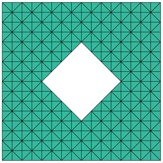
Figure 2. ${\Omega }_1$ : a rhomboidal tube with edge side length $2\sqrt{2}$ immersed in the square ${\left(-4,4\right)}^2$

图2. ${\Omega }_1$ ：边长为 $2\sqrt{2}$ 的菱形管浸没在方形腔 ${\left(-4,4\right)}^2$ 中

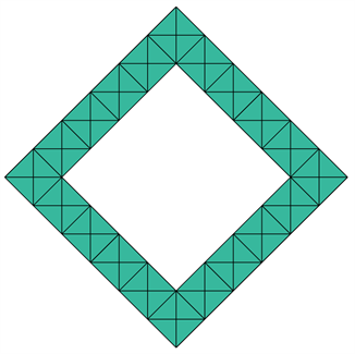
Figure 3. ${\Omega }_3$ : local correction domain on ${\Omega }_1$

图3. ${\Omega }_3$ ：在 ${\Omega }_1$ 上的局部校正区域

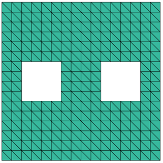
Figure 4. ${\Omega }_2$ : two square tubes with side length 2 immersed in a square cavity ${\left(-4,4\right)}^2$

图4. ${\Omega }_2$ ：两个边长为2的方管浸没在方形腔 ${\left(-4,4\right)}^2$ 中

Figure 5. ${\Omega }_4$ : local correction domain on ${\Omega }_2$

图5. ${\Omega }_4$ ：在 ${\Omega }_2$ 上的局部校正区域

Table 1. The approximation of the smallest eigenvalue obtained by Scheme 1 on Ω 1

表1. 由方案1求得的 ${\Omega }_1$ 上最小特征值的近似值

Table 2. The approximation of the first eigenvalue on Ω 2 obtained by parallel scheme

表2. 由并行计算方案求得的 ${\Omega }_2$ 上最小特征值的近似值

Table 3. The approximation of the second eigenvalue on Ω 2 obtained by parallel scheme

表3. 由并行计算方案求得的 ${\Omega }_2$ 上第二个特征值的近似值

Table 4. The approximation of the third eigenvalue on Ω 2 obtained by parallel scheme

表4. 由并行计算方案求得的 ${\Omega }_2$ 上第三个特征值的近似值

Table 5. The approximation of the fourth eigenvalue on Ω 2 obtained by parallel scheme

表5. 由并行计算方案求得的 ${\Omega }_2$ 上第四个特征值的近似值