两个随机相关的新古典增长模型的稳定性

Stability of Stochastic Two Connected Neoclassical Growth Models

摘要: 本文的目的是研究两个受白噪声影响的随机新古典增长模型的零平衡点稳定性。通过李雅普诺夫函数和Itô’s公式，得到了该模型的指数均方稳定性的新条件。最后，我们给出了两个例子来解释得到的结果。

Abstract: In this paper, our aim is to investigate the stability of the zero equilibrium point of stochastic two connected neoclassical growth models affected by white noise. By the aid of Lyapunov functional and Itô’s formula, we obtain a new condition on the exponentially mean square stable of this model. Finally, we give two examples to explain our result.

1. 绪论

众所周知，时滞微分新古典增长模型由于在数学经济学中的重要应用而受到了广泛的关注。许多研究者对研究这种模型有极大兴趣，有一些文件我们可以参考 [1] [2] [3] [4]。一般来说，噪声对系统有重要的影响，它可能使一个系统稳定也能够使一个系统不稳定。因此，受白噪声影响的系统是值得考虑的。据我们所知，已经有一些关于这一研究课题的文章。例如， [5] 研究了随机时滞微分方程的指数稳定性的鲁棒性。 [6] 利用线性矩阵不等式(LMI’S)技术研究了具有时滞和非线性不确定性的随机系统的时滞相关鲁棒稳定性。 [7] 利用Lyapunov-Krasovskii泛函方程和LMI混合延迟的微分方程，讨论了一类脉冲非线性随机方程的指数稳定性。 [8] 研究了随机非线性延迟动力系统的稳定性。此外，Shaikhet研究了一些关于受噪声影响的系统稳定性。例如， [9] 考虑了一个受白噪声影响的具有指数和二次非线性的非线性微分方程。 [10] 讨论了关于随机扰动时滞微分新古典增长模型的平衡点在受到白噪声类型的随机扰动影响下的稳定性分析。 [11] 通过利用LMI矩阵的方法研究两个相关的新古典增长模型在白噪声影响下的稳定性分析。基于 [11]，本文仍然考虑受到白噪声随机扰动下的两个连接的新古典生长模型零平衡点的稳定性。我们虽方法比较古老，但是却也得到一个不同于Shaikhet的零解稳定判别式。其实，我们没有用线性矩阵不等式去计算的原因主要也是因为考虑到在此情况下，用不等式的性质就可以解决模型中的交叉项，但是此方法比较古老，不一定适用于所有的新型动力系统模型，所以在本文定理证明那里我们可以看到，我们的主要工作就是找到此模型下满足判别条件的参数值。

首先，我们给出了一个两个相关的时滞差分新古典增长模型组成的系统，模型如下：

${\stackrel{\dot{}}{x}}_1\left(t\right)=a_1{x}_1^{{\gamma }_1}\left(t-h_1\right){\text{e}}^{-{\delta }_1{x}_1\left(t-h_1\right)}+b_1{x}_2\left(t\right)-c_1{x}_1\left(t\right)+{\sigma }_1\left(x_1\left(t\right)-x_1^{*}\right){\stackrel{\dot{}}{w}}_1\left(t\right),$

${\stackrel{\dot{}}{x}}_2\left(t\right)=a_2{x}_2^{{\gamma }_2}\left(t-h_2\right){\text{e}}^{-{\delta }_2{x}_2\left(t-h_2\right)}+b_2{x}_1\left(t\right)-c_2{x}_2\left(t\right)+{\sigma }_2\left(x_2\left(t\right)-x_2^{*}\right){\stackrel{\dot{}}{w}}_2\left(t\right),$

$x_i\left(s\right)={\varphi }_i\left(s\right),s\in \left[-h_i,0\right],i=1,2,$ (1.1)

这里 $a_i,b_i,c_i,{\delta }_i$ 是正的参数， ${\gamma }_i\ge 1,h_i\ge 0,i=1,2$。 ${\sigma }_1,{\sigma }_2$ 是常数， $w_1\left(t\right),w_2\left(t\right)$ 是相互独立的标准Wiener过程， $\left(x_1^{*},x_2^{*}\right)$ 是系统(1.1)的平衡点。

本文由以下几部分组成。在第二节中，我们做了一些准备工作为本文的使用。在第三节中，我们给出了两个随机新古典增长模型的零平衡点是指数均方稳定的条件。在第四节中，我们用两个例子来验证得到的结果。

2. 准备工作

使用新的变量 $y_i\left(t\right)=x_i\left(t\right)-x_i^{*}$，我们中心化系统(1.1)并且得到

$\begin{array}{l}{\stackrel{\dot{}}{y}}_1\left(t\right)=-c_1{y}_1\left(t\right)+a_1{\text{e}}^{-{\delta }_1{x}_1^{*}}\left[{\left(y_1\left(t-h_1\right)+x_1^{*}\right)}^{{\gamma }_1}{\text{e}}^{-{\delta }_1{y}_1\left(t-h_1\right)}-{\left(x_1^{*}\right)}^{{\gamma }_1}\right]+b_1{y}_2\left(t\right)+{\sigma }_1{y}_1\left(t\right){\stackrel{\dot{}}{w}}_1\left(t\right),\\ {\stackrel{\dot{}}{y}}_2\left(t\right)=-c_2{y}_2\left(t\right)+a_2{\text{e}}^{-{\delta }_2{x}_2^{*}}\left[{\left(y_2\left(t-h_2\right)+x_2^{*}\right)}^{{\gamma }_2}{\text{e}}^{-{\delta }_2{y}_2\left(t-h_2\right)}-{\left(x_2^{*}\right)}^{{\gamma }_2}\right]+b_2{y}_1\left(t\right)+{\sigma }_2{y}_2\left(t\right){\stackrel{\dot{}}{w}}_2\left(t\right),\end{array}$ (2.1)

接下来，令 ${\mu }_i={\delta }_i{x}_i^{*}-{\gamma }_i,i=1,2$，我们得到了非线性系统(2.1)的线性部分如下 [12]：

$\begin{array}{l}{\stackrel{\dot{}}{z}}_1\left(t\right)=-c_1{z}_1\left(t\right)+b_1{z}_2\left(t\right)\left(b_1{x}_2^{*}/x_1^{*}-c_1\right){\mu }_1{z}_1\left(t-h_1\right)+{\sigma }_1{z}_1\left(t\right){\stackrel{\dot{}}{w}}_1\left(t\right),\\ {\stackrel{\dot{}}{z}}_2\left(t\right)=-c_2{z}_2\left(t\right)+b_2{z}_1\left(t\right)\left(b_2{x}_1^{*}/x_2^{*}-c_2\right){\mu }_2{z}_2\left(t-h_2\right)+{\sigma }_2{z}_2\left(t\right){\stackrel{\dot{}}{w}}_2\left(t\right),\end{array}$ (2.2)

引理2.1 [10] 函数 $f\left(x\right)=x^{{\gamma }_i-1}{\text{e}}^{-{\delta }_{i}x},x\ge 0,{\gamma }_i\ge 1,{\delta }_i>0$，满足条件 $\underset{x\ge 0}{\sup }f\left(x\right)=K_i$，其中如果 ${\gamma }_i>1$，

$K_i={\left(\frac{{\gamma }_i-1}{e{\delta }_i}\right)}^{{\gamma }_i-1}$，并且 ${\gamma }_i=1$，。

设L为系统(2.1)的算子 [12]， $y\left(t\right)$ 是(2.1)在时间t的解， $y_t$ 是(2.1)直到时间矩t的解的轨迹。 $h=h_1\vee h_2$，E是期望。

定义2.1 系统(2.1)的初值为 $y\left(s\right)=\varphi \left(s\right),s\in \left[-h,0\right]$，其零解是指数均方稳定的如果存在一对常数 $\lambda$ 和C使得

$E{\left|y\left(t,\varphi \right)\right|}^2\le CE{\left|\varphi \right|}^2{\text{e}}^{-\lambda t},t\ge 0.$

定理2.1 [13] 设存在一个函数 $V\left(t,\varphi \right)$ 且 $\lambda >0$ 使得对于系统(2.1)的解 $y\left(t\right)$ 满足：

$EV\left(t,y_t\right)\ge q_1{\text{e}}^{\lambda t}E{\left|y\left(t\right)\right|}^2,$

$EV\left(0,\varphi \right)\le q_2{\Vert \varphi \Vert }^2,$

$ELV\left(t,y_t\right)\le 0,t\ge 0,q_1,q_2>0.$

则系统(2.1)的零解是指数均方稳定的，其中， ${\Vert \varphi \Vert }^2=\underset{s\le 0}{\sup }E{\left|\varphi \left(s\right)\right|}^2$。

3. 两个随机相关的新古典增长模型的稳定性

以下是系统(2.1)的零平衡点模型。

$\begin{array}{l}{\stackrel{\dot{}}{y}}_1\left(t\right)=-c_1{y}_1\left(t\right)+b_1{y}_2\left(t\right)+a_1{y}_1^{{\gamma }_1}\left(t-h_1\right){\text{e}}^{-{\delta }_1{y}_1\left(t-h_1\right)}+{\sigma }_1{y}_1\left(t\right){\stackrel{\dot{}}{w}}_1\left(t\right),\\ {\stackrel{\dot{}}{y}}_2\left(t\right)=-c_2{y}_2\left(t\right)+b_2{y}_1\left(t\right)+a_2{y}_2^{{\gamma }_2}\left(t-h_2\right){\text{e}}^{-{\delta }_2{y}_2\left(t-h_2\right)}+{\sigma }_2{y}_2\left(t\right){\stackrel{\dot{}}{w}}_2\left(t\right),\end{array}$ (3.1)

假设3.1 对于正数 $d_1,d_2$ 和 $\lambda \ge 0$，下面的不等式成立：

$d_1\left(\lambda -2c_1+{\sigma }_1^2+a_1{K}_1+a_1{K}_1{\text{e}}^{\lambda h_1}\right)+d_1{b}_1+d_2{b}_2<0,$

$d_2\left(\lambda -2c_2+{\sigma }_2^2+a_2{K}_2+a_2{K}_2{\text{e}}^{\lambda h_2}\right)+d_1{b}_1+d_2{b}_2<0.$

定理3.1如果系统(2.2)满足假设3.1，则系统(2.2)的零平衡点是指数均方稳定的。

证明：首先构造李雅普诺夫泛函 $V_1\left(t,y\left(t\right)\right)={\text{e}}^{\lambda t}{\displaystyle \underset{i=1}{\overset{2}{\sum }}{d}_i}{y}_i^2\left(t\right)$，然后我们有

$\begin{array}{c}L{V}_1\left(t,y\left(t\right)\right)={\text{e}}^{\lambda t}[\lambda {\displaystyle \underset{i=1}{\overset{2}{\sum }}{d}_i}{y}_i^2\left(t\right)+2d_1{y}_1\left(t\right)\left(a_1{y}_1^{{\gamma }_1}\left(t-h_1\right){\text{e}}^{-{\delta }_1{y}_1\left(t-h_1\right)}-c_1{y}_1\left(t\right)\right)+d_1{\sigma }_1^2{y}_1^2\left(t\right)\\ \begin{array}{c}\\ \end{array}+b_1{y}_2\left(t\right)+2d_2{y}_2\left(t\right)\left(b_2{y}_1\left(t\right)+a_2{y}_2^{{\gamma }_2}\left(t-h_2\right){\text{e}}^{-{\delta }_2{y}_2\left(t-h_2\right)}-c_2{y}_2\left(t\right)\right)+d_2{\sigma }_2^2{y}_2^2\left(t\right)]\\ ={\text{e}}^{\lambda t}[\lambda {\displaystyle \underset{i=1}{\overset{2}{\sum }}{d}_i}{y}_i^2\left(t\right)-2{\displaystyle \underset{i=1}{\overset{2}{\sum }}{d}_i}{c}_i{y}_i^2\left(t\right)+2\left(d_1{b}_1+d_2{b}_2\right)y_1\left(t\right)y_2\left(t\right)\\ +{\displaystyle \underset{i=1}{\overset{2}{\sum }}{d}_i}{\sigma }_i^2{y}_i^2\left(t\right)+2{\displaystyle \underset{i=1}{\overset{2}{\sum }}{d}_i}{a}_i{y}_i\left(t\right)y_i^{{\gamma }_i}\left(t-h_i\right){\text{e}}^{-{\delta }_i{y}_i\left(t-h_i\right)}]\\ \le {\text{e}}^{\lambda t}[{\displaystyle \underset{i=1}{\overset{2}{\sum }}{d}_i}\left(\lambda -2c_i+{\sigma }_i^2+a_i{K}_i\right)y_i^2\left(t\right)+\left(d_1{b}_1+d_2{b}_2\right)y_1^2\left(t\right)\\ +\left(d_1{b}_1+d_2{b}_2\right)y_2^2\left(t\right)+{\displaystyle \underset{i=1}{\overset{2}{\sum }}{d}_i}{a}_i{K}_i{y}_i^2\left(t-h_i\right)]\end{array}$

令 $V_2\left(t,y_t\right)={\displaystyle \underset{i=1}{\overset{2}{\sum }}{d}_i}{a}_i{K}_i{\displaystyle {\int }_{t-h_i}^t{\text{e}}^{\lambda \left(s+h_i\right)}}{y}_i^2\left(s\right)\text{d}s$，因此，我们获得

$L{V}_2\left(t,y_t\right)={\text{e}}^{\lambda t}{\displaystyle \underset{i=1}{\overset{2}{\sum }}{d}_i}{a}_i{K}_i\left({\text{e}}^{\lambda h_i}{y}_i^2\left(t\right)-y_i^2\left(t-h_i\right)\right)$

设 $V\left(t,y_t\right)=V_1\left(t,y\left(t\right)\right)+V_2\left(t,y_t\right)$，然后有

$\begin{array}{c}LV\left(t,y_t\right)\le {\text{e}}^{\lambda t}[{\displaystyle \underset{i=1}{\overset{2}{\sum }}{d}_i\left(\lambda -2c_i+{\sigma }_i^2+a_i{K}_i+a_i{K}_i{\text{e}}^{\lambda h_i}\right)y_i^2\left(t\right)}+\left(d_1{b}_1+d_2{b}_2\right)y_1^2\left(t\right)\\ +\left(d_1{b}_1+d_2{b}_2\right)y_2^2\left(t\right)+{\displaystyle \underset{i=1}{\overset{2}{\sum }}{d}_i}{a}_i{K}_i{y}_i^2\left(t-h_i\right)]\\ ={\text{e}}^{\lambda t}[d_1\left(\lambda -2c_1+{\sigma }_1^2+a_1{K}_1+a_1{K}_1{\text{e}}^{\lambda h_1}\right)y_1^2\left(t\right)+\left(d_1{b}_1+d_2{b}_2\right)y_1^2\left(t\right)\\ +d_2\left(\lambda -2c_2+{\sigma }_2^2+a_2{K}_2+a_2{K}_2{\text{e}}^{\lambda h_2}\right)y_2^2\left(t\right)+\left(d_1{b}_1+d_2{b}_2\right)y_2^2\left(t\right)]\\ ={\text{e}}^{\lambda t}[\left(d_1\left(\lambda -2c_1+{\sigma }_1^2+a_1{K}_1+a_1{K}_1{\text{e}}^{\lambda h_1}\right)+d_1{b}_1+d_2{b}_2\right)y_1^2\left(t\right)\\ +\left(d_2\left(\lambda -2c_2+{\sigma }_2^2+a_2{K}_2+a_2{K}_2{e}^{\lambda h_2}\right)+d_1{b}_1+d_2{b}_2\right)y_2^2\left(t\right)]\end{array}$

通过假设3.1，我们得到 $LV\left(t,y_t\right)<0$。

$\begin{array}{c}EV\left(0,\varphi \right)={\displaystyle \underset{i=1}{\overset{2}{\sum }}{d}_{i}E{\varphi }_i^2\left(0\right)}+{\displaystyle \underset{i=1}{\overset{2}{\sum }}{d}_i}{a}_i{K}_i{\displaystyle {\int }_{-h_i}^{0}E{\text{e}}^{\lambda \left(s+h_i\right)}{\varphi }_i^2}\left(s\right)\text{d}s\\ \le \left(d_1\vee d_2\right){\displaystyle \underset{i=1}{\overset{2}{\sum }}E{\varphi }_i^2\left(0\right)}+\left(d_1{a}_1{K}_1\vee d_2{a}_2{K}_2\right){\displaystyle {\int }_{-h_i}^{0}E{\text{e}}^{\lambda \left(s+h_i\right)}}{\varphi }_i^2\left(s\right)\text{d}s\\ \le \left[\left(d_1\vee d_2\right)+\left(d_1{a}_1{K}_1\vee d_2{a}_2{K}_2\right)\right]{\Vert \varphi \Vert }^2\end{array}$

根据李雅普诺夫函数 $V\left(t,y_t\right)$ 的形式，我们

$EV\left(t,y_t\right)\ge E{\text{e}}^{\lambda t}{\displaystyle \underset{i=1}{\overset{2}{\sum }}{d}_i}{y}_i^2\left(t\right)\ge \left(d_1\wedge d_2\right){\text{e}}^{\lambda t}E{\left|y\left(t\right)\right|}^2.$

因此，根据定理2.1，系统(2.2)的零平衡点是指数均方稳定的。

4. 实例

在本节中，我们的任务是验证结果。

例1：考虑系统(3.1)，我们为这两个方程选择了相同的参数，即，

$\begin{array}{l}{a}_1=50,a_2=50,b_1=32,b_2=32,c_1=60,c_2=60,{\gamma }_1=3,{\gamma }_2=3,{\delta }_1=1,{\delta }_2=1,\\ h_1=0.06,h_2=0.06,{\sigma }_1=1,{\sigma }_2=1,d_1=0.0516,d_2=0.0516,\lambda =0.\end{array}$

通过引理2.1，我们有

$K_1={\left(\frac{{\gamma }_1-1}{e{\delta }_1}\right)}^{{\gamma }_1-1}=0.5413,$

$K_2={\left(\frac{{\gamma }_2-1}{e{\delta }_2}\right)}^{{\gamma }_2-1}=\mathrm{0.5413.}$

接下来，我们计算

$d_1\left(\lambda -2c_1+{\sigma }_1^2+a_1{K}_1+a_1{K}_1{\text{e}}^{\lambda h_1}\right)+d_1{b}_1+d_2{b}_2=-0.0449<0,$

$d_2\left(\lambda -2c_2+{\sigma }_2^2+a_2{K}_2+a_2{K}_2{\text{e}}^{\lambda h_2}\right)+d_1{b}_1+d_2{b}_2=-0.0449<0.$

因此，通过定理3.1，系统(3.1)是指数均方稳定的。然而，如果选择 $b_1=41,b_2=41$ 并且其它参数保持不变。那么

$d_1\left(\lambda -2c_1+{\sigma }_1^2+a_1{K}_1+a_1{K}_1{\text{e}}^{\lambda h_1}\right)+d_1{b}_1+d_2{b}_2=0.8839>0,$

$d_2\left(\lambda -2c_2+{\sigma }_2^2+a_2{K}_2+a_2{K}_2{\text{e}}^{\lambda h_2}\right)+d_1{b}_1+d_2{b}_2=0.8839>0.$

也就是说，系统(3.1)是不稳定的。我们取 $y_1\left(t\right)$ 和 $y_2\left(t\right)$ 的初始值为 $y_1\left(s\right)=0.35\cos \left(20s\right)$， $y_2\left(s\right)=1.65\cos \left(20s\right)$， $s\in \left[-0.06,0\right]$。根据第一组参数，我图们做出了图1。证明了系统(3.1)的零解是指数均方稳定的。通过另一组数据，我们获得了图2并且表示系统(3.1)的零解是不稳定的。

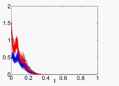
Figure 1. When $b_1=32,b_2=32$ the zero solution is exponentially mean-square stable

图1. 当 $b_1=32,b_2=32$ 时，零解呈现指数均方稳定

Figure 2. When $b_1=41,b_2=41$, the zero solution is unstable

图2. 当 $b_1=41,b_2=41$ 时，零解不稳定

例2：考虑系统(3.1)，我们选择不同参数的两个方程的：

$\begin{array}{l}{a}_1=30,a_2=20,b_1=10,b_2=10,c_1=35,c_2=30,{\gamma }_1=2,{\gamma }_2=3,{\delta }_1=1,{\delta }_2=1,\\ h_1=0.06,h_2=0.06,{\sigma }_1=1,{\sigma }_2=1,d_1=0.0289,d_2=0.0319,\lambda =1.\end{array}$

根据引理2.1，我们有

$K_1={\left(\frac{{\gamma }_1-1}{e{\delta }_1}\right)}^{{\gamma }_1-1}=0.3679,$

$K_2={\left(\frac{{\gamma }_2-1}{e{\delta }_2}\right)}^{{\gamma }_2-1}=\mathrm{0.5413.}$

然后，我们得到

$d_1\left(\lambda -2c_1+{\sigma }_1^2+a_1{K}_1+a_1{K}_1{e}^{\lambda h_1}\right)+d_1{b}_1+d_2{b}_2=-0.6995<0,$

$d_2\left(\lambda -2c_2+{\sigma }_2^2+a_2{K}_2+a_2{K}_2{\text{e}}^{\lambda h_2}\right)+d_1{b}_1+d_2{b}_2=-0.5301<0.$

因此，通过定理3.1，系统(3.1)是指数均方稳定的。令 $b_1=25,b_2=25$ 并且其它参数保持不变。这样，

$d_1\left(\lambda -2c_1+{\sigma }_1^2+a_1{K}_1+a_1{K}_1{\text{e}}^{\lambda h_1}\right)+d_1{b}_1+d_2{b}_2=0.2125>0,$

$d_2\left(\lambda -2c_2+{\sigma }_2^2+a_2{K}_2+a_2{K}_2{\text{e}}^{\lambda h_2}\right)+d_1{b}_1+d_2{b}_2=0.3819>0.$

结果表明，系统(3.1)是不稳定的。通过选取的参数我们做出了图3和图4。

Figure 3. When $b_1=10,b_2=10$, system(3.1) is exponentially mean-square stable

图3. 当 $b_1=10,b_2=10$ 时，系统(3.1)指数均方稳定

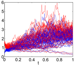
Figure 4. When $b_1=25,b_2=25$, system (3.1) is unstable

图4. 当 $b_1=25,b_2=25$ 时，系统(3.1)不稳定

从图3中我们可以看到，系统(3.1)的零解是指数均方稳定的。然而，图4表明系统(3.1)的零解是不稳定的。

这两个例子表明，选择合适的耦合系数 $\left(b_1,b_2\right)$ 对于系统的稳定性是非常重要的。

参考文献