一类时滞BAM神经网络的全局渐近同步

Global Asymptotic Synchronization for a Class of BAM Neural Networks with Time Delays

摘要: 本文考虑一类时滞BAM神经网络系统的全局渐近同步问题。利用Lyapunov泛函和分析方法，给出了两个能够保证所考虑系统的全局渐近同步的充分判据，所得结果一定程度上比本文的主要参考文献有较为广泛的适应性。

Abstract: In this paper, the global asymptotic synchronization of a class of BAM neural networks with time delays is considered. By using the Lyapunov functionals and analytical methods, two sufficient criteria are given to ensure the global asymptotic synchronization of our system. To some extent, the present results are more feasible than the main reference in this paper.

1. 引言

神经网络是一类基于模拟生物神经系统得出的数学模型，它可用于实现类似生物神经系统储存和处理信息的功能 [1]。BAM神经网络是当中一类具有记忆、储存、联想功能的联想记忆神经网络，它是由Kosko在1987年首次提出并研究的神经网络模型 [2] [3]。这类神经网络是由两层(X-层，Y-层)非线性反馈网络以二分图的形式组成的，即X-层的神经元和Y-层的神经元完全互连，同一层的神经元之间不存在任何连接 [1]。由于 BAM 神经网络有信息联想记忆和储存双极向量对的能力，这类神经网络被运用到了诸多领域，如图像信号处理 [4]、联想记忆 [5]、模式识别 [6]、自动控制 [7]、最优化问题 [8] 等方面。另外，由于神经网络系统在信号传输和切换过程中会不可避免地存在时滞现象，因此，研究具有时滞的神经网络具有更为广泛的意义 [9] - [15]。

在研究神经网络数学模型的性态方面，模型的稳定性一直是人们关注的热点，因为它涉及到实际应用中的诸如模式识别的可靠性、输入状态对输出状态的影响等 [9]。在众多的神经网络稳定性研究中，我们注意到，渐近同步话题引起了研究者的广泛关注 [10] - [15]。神经网络系统同步的研究，不仅给安全通信 [10]、信息科学 [11]、图像处理 [12] 提供了理论基础，而且对基础科学也有重要影响。近些年，关于时滞BAM神经网络系统的同步问题研究，普遍做法是利用Lyapunov泛函，结合线性矩阵不等式(LMI)或积分不等式 [13] [14]，或者矩阵测度的方法 [15]。这里，我们特别注意的是，文献 [14] 考虑了时滞BAM神经网络：

$\{\begin{array}{l}{x^{\prime }}_i\left(t\right)=-{\alpha }_i{x}_i\left(t\right)+{\displaystyle {\sum }_{j=1}^m{a}_{ij}{f}_j\left(y_j\left(t\right)\right)}+{\displaystyle {\sum }_{j=1}^m{p}_{ij}{f}_j\left(y_j\left(t-{\tau }_{ji}\right)\right)}+I_i,\\ {y^{\prime }}_j\left(t\right)=-{\beta }_j{y}_j\left(t\right)+{\displaystyle {\sum }_{i=1}^n{b}_{ji}{g}_i\left(x_i\left(t\right)\right)}+{\displaystyle {\sum }_{i=1}^n{q}_{ji}{g}_i\left(x_i\left(t-{\bar{\tau }}_{ij}\right)\right)}+J_j,\\ i=1,2,\cdots ,n;j=1,2,\cdots ,m\end{array}$ (1.1)

以及它的扰动系统

$\{\begin{array}{l}{u^{\prime }}_i\left(t\right)=-{\alpha }_i{u}_i\left(t\right)+{\displaystyle {\sum }_{j=1}^m{a}_{ij}{f}_j\left(v_j\left(t\right)\right)}+{\displaystyle {\sum }_{j=1}^m{p}_{ij}{f}_j\left(v_j\left(t-{\tau }_{ji}\right)\right)}+I_i+P_i\left(t\right),\\ {v^{\prime }}_j\left(t\right)=-{\beta }_j{v}_j\left(t\right)+{\displaystyle {\sum }_{i=1}^n{b}_{ji}{g}_i\left(u_i\left(t\right)\right)}+{\displaystyle {\sum }_{i=1}^n{q}_{ji}{g}_i\left(u_i\left(t-{\bar{\tau }}_{ij}\right)\right)}+J_j+Q_j\left(t\right),\\ i=1,2,\cdots ,n;j=1,2,\cdots ,m\end{array}$ (1.2)

其中常数 ${\alpha }_i$， ${\beta }_j$ 表示神经元的负载时间常数和被动衰变率； $f_j$， $g_j$ 表示神经元的激活函数；常数 $a_{ij}$， $p_{ij}$， $b_{ji}$， $q_{ji}$ 表示第i个神经元和第j个神经元之间的轴突联络强度(连接权值)； ${\tau }_{ji}$， ${\bar{\tau }}_{ij}$ 是时滞参数； $I_i$， $J_j$ 是外部常值输入； $x_i\left(t\right)$， $y_j\left(t\right)$ 和 $u_i\left(t\right)$， $v_j\left(k\right)$ 分别表示t时刻的神经元的状态变量。

文献 [14] 将(1.1)称为驱动系统，(1.2)称为响应系统； $P_i\left(t\right)$， $Q_j\left(t\right)$ 被称为控制器，用于实现驱动系统和响应系统的全局渐近同步。为了这个目的，文献 [14] 引入了条件

(H0) $\underset{1\le j\le m}{\max }\left\{-{\beta }_j\right\}<\underset{1\le i\le n}{\max }\left\{-{\alpha }_i\right\}<0$。

那么，我们的疑问是，能否在没有(H0)约束的情况下，系统(1.1)和(1.2)仍然全局渐近同步？这是本文的思考动因。我们发现，借鉴文献 [9] [14] 的方法，这个问题可以得到肯定的回答。

下面讨论中，我们假设

(H1) $f_j$ 、 $g_i$ 都是连续函数，且存在非负常数 $F_j$ 、 $G_i$，使得对一切的 ${\omega }_1,{\omega }_2\in ℝ$， $i=1,2,\cdots ,n$， $j=1,2,\cdots ,m$，有

$\left|f_j\left({\omega }_1\right)-f_j\left({\omega }_2\right)\right|\le F_j\left|{\omega }_1-{\omega }_2\right|$， $\left|g_i\left({\omega }_1\right)-g_i\left({\omega }_2\right)\right|\le G_i\left|{\omega }_1-{\omega }_2\right|$ ；

(H2)

$\eta =\underset{1\le i\le n,1\le j\le m}{\min }\left\{-{\alpha }_i+{\displaystyle {\sum }_{j=1}^m{G}_i}\left(\left|b_{ji}\right|+\left|q_{ji}\right|\right),-{\beta }_j+{\displaystyle {\sum }_{i=1}^n{F}_j\left(\left|a_{ij}\right|+\left|p_{ij}\right|\right)}\right\}>0$

$\mu =\underset{1\le i\le n,1\le j\le m}{\min }\left\{{\alpha }_i,{\beta }_j\right\}>0$

$\lambda =\underset{1\le i\le n,1\le j\le m}{\min }\left\{-{\displaystyle {\sum }_{j=1}^m\left(\left|b_{ji}\right|+\left|q_{ji}\right|\right)G_i},-{\displaystyle {\sum }_{i=1}^n\left(\left|a_{ij}\right|+\left|p_{ij}\right|\right)F_j}\right\}$

下面我们用 $\left(x\left(t\right),y\left(t\right)\right)$ 、 $\left(u\left(t\right),v\left(t\right)\right)$ 分别表示系统(1.1)和(1.2)的解。

定义1 [14] 若系统(1.1)的任意解 $\left(x\left(t\right),y\left(t\right)\right)$ 和系统(1.2)的任意解 $\left(u\left(t\right),v\left(t\right)\right)$ 满足：

$\underset{t\to \infty }{\lim }\left|u_i\left(t\right)-x_i\left(t\right)\right|=0$

$\underset{t\to \infty }{\lim }\left|v_j\left(t\right)-y_j\left(t\right)\right|=0$

则称系统(1.1)和(1.2)全局渐近同步。

2. 主要结论

记 $e_i\left(t\right)=u_i\left(t\right)-x_i\left(t\right)$， $r_j\left(t\right)=v_j\left(t\right)-y_j\left(t\right)$，则

$\{\begin{array}{l}{e^{\prime }}_i\left(t\right)=-{\alpha }_i{e}_i\left(t\right)+{\displaystyle {\sum }_{j=1}^m{a}_{ij}\left[f_j\left(v_j\left(t\right)\right)-f_j\left(y_j\left(t\right)\right)\right]}\\ +{\displaystyle {\sum }_{j=1}^m{p}_{ij}\left[f_j\left(v_j\left(t-{\tau }_{ji}\right)\right)-f_j\left(y_j\left(t-{\tau }_{ji}\right)\right)\right]}+P_i\left(t\right),\\ {r^{\prime }}_j\left(t\right)=-{\beta }_j{r}_j\left(t\right)+{\displaystyle {\sum }_{i=1}^n{b}_{ji}\left[g_i\left(u_i\left(t\right)\right)-g_i\left(x_i\left(t\right)\right)\right]}\\ +{\displaystyle {\sum }_{i=1}^n{q}_{ji}\left[g_i\left(u_i\left(t-{\bar{\tau }}_{ij}\right)\right)-g_i\left(x_i\left(t-{\bar{\tau }}_{ij}\right)\right)\right]}+Q_j\left(t\right),\\ i=1,2,\cdots ,n;j=1,2,\cdots ,m\end{array}$ (2.1)

这样，系统(1.1)和(1.2)的全局渐近同步问题，等价于

$\underset{t\to \infty }{\lim }\left(e\left(t\right),r\left(t\right)\right)=\left(0,0\right)$

定理1：假设条件(H1)和(H2)成立， $P\left(t\right)=(P_1\left(t\right),P_2\left(t\right),{\cdots ,P_n\left(t\right))}^{\text{T}}$， $Q\left(t\right)=(Q_1\left(t\right),Q_2\left(t\right),\cdots ,{Q_m\left(t\right))}^{\text{T}}$ 满足：

${\displaystyle {\int }_0^{\infty }{\displaystyle {\sum }_{i=1}^n\left|P_i\left(s\right)\right|}+{\displaystyle {\sum }_{j=1}^m\left|Q_j\left(s\right)\right|\text{d}s}}<\infty$ (2.2)

则系统(1.1)和(1.2)全局渐近同步，即

$\underset{t\to \infty }{\lim }\left|u_i\left(t\right)-x_i\left(t\right)\right|=0$,

$\underset{t\to \infty }{\lim }\left|v_j\left(t\right)-y_j\left(t\right)\right|=0$.

证明：首先，基于(2.1)，我们定义如下的Lyapunov函数 $V\left[e,r\right]\left(t\right):ℝ\to ℝ$ ：

$\begin{array}{l}V\left[e,r\right]\left(t\right)={\displaystyle {\sum }_{i=1}^n{e}_i\left(t\right)}+{\displaystyle {\sum }_{j=1}^m{r}_j\left(t\right)}\\ +{\displaystyle {\sum }_{i=1}^n{\displaystyle {\sum }_{j=1}^m\left|p_{ij}\right|}\left|{\displaystyle {\int }_{t-{\tau }_{ji}}^t{f}_j\left(v_j\left(s\right)\right)-f_j\left(y_j\left(s\right)\right)\text{d}s}\right|}\\ +{\displaystyle {\sum }_{j=1}^m{\displaystyle {\sum }_{i=1}^n\left|q_{ji}\right|}\left|{\displaystyle {\int }_{t-{\bar{\tau }}_{ij}}^t{g}_i\left(u_i\left(s\right)\right)-g_i\left(x_i\left(s\right)\right)\text{d}s}\right|}\end{array}$

这里，我们简记函数 $V\left[e,r\right]\left(t\right)$ 为 $V\left(t\right)$。沿着系统 的解， $V\left(t\right)$ 的右上导数为：

$\begin{array}{l}{D}^{+}V\left(t\right)={\displaystyle {\sum }_{i=1}^n\mathrm{sgn}{e}_i\left(t\right)\{-{\alpha }_i{e}_i\left(t\right)+{\displaystyle {\sum }_{j=1}^m{a}_{ij}\left[f_j\left(v_j\left(t\right)\right)-f_j\left(y_j\left(t\right)\right)\right]}}\\ +{\displaystyle {\sum }_{j=1}^m{p}_{ij}\left[f_j\left(v_j\left(t-{\tau }_{ji}\right)\right)-f_j\left(y_j\left(t-{\tau }_{ji}\right)\right)\right]}+P_i\left(t\right)\}\\ +{\displaystyle {\sum }_{j=1}^m\mathrm{sgn}{r}_j\left(t\right)\{-{\beta }_j{r}_j\left(t\right)+{\displaystyle {\sum }_{i=1}^n{b}_{ji}\left[g_i\left(u_i\left(t\right)\right)-g_i\left(x_i\left(t\right)\right)\right]}}\\ +{\displaystyle {\sum }_{j=1}^m{q}_{ji}\left[g_i\left(u_i\left(t-{\bar{\tau }}_{ij}\right)\right)-g_i\left(x_i\left(t-{\bar{\tau }}_{ij}\right)\right)\right]}+Q_j\left(t\right)\}\\ +{\displaystyle {\sum }_{i=1}^n{\displaystyle {\sum }_{j=1}^m\left|p_{ij}\right|\left[\left|f_j\left(v_j\left(t\right)\right)-f_j\left(y_j\left(t\right)\right)\right|-\left|f_j\left(v_j\left(t-{\tau }_{ji}\right)\right)-f_j\left(y_j\left(t-{\tau }_{ji}\right)\right)\right|\right]}}\end{array}$

$\begin{array}{l}+{\displaystyle {\sum }_{j=1}^m{\displaystyle {\sum }_{i=1}^n\left|q_{ji}\right|\left[\left|g_i\left(u_i\left(t\right)\right)-g_i\left(x_i\left(t\right)\right)\right|-\left|g_i\left(u_i\left(t-{\bar{\tau }}_{ij}\right)\right)-g_i\left(x_i\left(t-{\bar{\tau }}_{ij}\right)\right)\right|\right]}}\\ \le {\displaystyle {\sum }_{i=1}^n\left[-{\alpha }_i\left|e_i\left(t\right)\right|+{\displaystyle {\sum }_{j=1}^m\left(\left|a_{ij}\right|+\left|p_{ij}\right|\right)\left|f_j\left(v_j\left(t\right)\right)-f_j\left(y_j\left(t\right)\right)\right|}\right]}\\ +{\displaystyle {\sum }_{j=1}^m\left[-{\beta }_j\left|r_j\left(t\right)\right|+{\displaystyle {\sum }_{i=1}^n\left(\left|b_{ji}\right|+\left|q_{ji}\right|\right)\left|g_i\left(u_i\left(t\right)\right)-g_i\left(x_i\left(t\right)\right)\right|}\right]}\\ +{\displaystyle {\sum }_{i=1}^n\left|P_i\left(t\right)\right|}+{\displaystyle {\sum }_{j=1}^m\left|Q_j\left(t\right)\right|}\end{array}$

由条件(H1)和(H2)可知

$\begin{array}{l}{D}^{+}V\left(t\right)\le {\displaystyle {\sum }_{i=1}^n\left[-{\alpha }_i+{\displaystyle {\sum }_{j=1}^m{G}_i\left(\left|b_{ji}\right|+\left|q_{ji}\right|\right)}\right]\left|e_i\left(t\right)\right|}\\ +{\displaystyle {\sum }_{j=1}^m\left[-{\beta }_j+{\displaystyle {\sum }_{i=1}^n{F}_j\left(\left|a_{ij}\right|+\left|p_{ij}\right|\right)}\right]\left|r_j\left(t\right)\right|}\\ +{\displaystyle {\sum }_{i=1}^n\left|P_i\left(t\right)\right|}+{\displaystyle {\sum }_{j=1}^m\left|Q_j\left(t\right)\right|}\\ \le -\eta \left({\displaystyle {\sum }_{i=1}^n\left|e_i\left(t\right)\right|}+{\displaystyle {\sum }_{j=1}^m\left|r_j\left(t\right)\right|}\right)+{\displaystyle {\sum }_{i=1}^n\left|P_i\left(t\right)\right|}+{\displaystyle {\sum }_{j=1}^m\left|Q_j\left(t\right)\right|}\end{array}$ (2.3)

于是，对不等式(2.3)两边从 $0$ 到 $t$ 积分可以得到

$V\left(t\right)+\eta {\displaystyle {\int }_0^t{\displaystyle {\sum }_{i=1}^n\left|e_i\left(s\right)\right|}+{\displaystyle {\sum }_{j=1}^m\left|r_j\left(s\right)\right|\text{d}s}}\le V\left(0\right)+{\displaystyle {\int }_0^t{\displaystyle {\sum }_{i=1}^n\left|P_i\left(s\right)\right|}+{\displaystyle {\sum }_{j=1}^m\left|Q_j\left(s\right)\right|\text{d}s}}$ (2.4)

注意到式(2.2)和 $V\left(0\right)$ 的有界性，由不等式(2.4)得知：

${\displaystyle {\int }_0^{\infty }{\displaystyle {\sum }_{i=1}^n\left|e_i\left(s\right)\right|}+{\displaystyle {\sum }_{j=1}^m\left|r_j\left(s\right)\right|\text{d}s}}<\infty$ (2.5)

$V\left(t\right)$ 在区间 $\left[0,\infty \right)$ 上有界

从而 $e_i\left(t\right),r_j\left(t\right)\left(i=1,2,\cdots ,n;j=1,2,\cdots ,m\right)$ 在区间 $\left[0,\infty \right)$ 有界。再由(2.1)、(2.2)可知 $e_i\left(t\right),r_j\left(t\right)$ 的导数在区间 $\left[0,\infty \right)$ 上有界，所以函数 $e_i\left(t\right),r_j\left(t\right)$ 在区间 $\left[0,\infty \right)$ 上一致连续。这样，再利用(2.5)，我们得到

$\underset{t\to \infty }{\lim }\left|e_i\left(t\right)\right|=\underset{t\to \infty }{\lim }\left|u_i\left(t\right)-x_i\left(t\right)\right|=0$

$\underset{t\to \infty }{\lim }\left|r_j\left(t\right)\right|=\underset{t\to \infty }{\lim }\left|v_j\left(t\right)-y_j\left(t\right)\right|=0$

即，系统(1.1)和(1.2)全局渐近同步。证毕。

下面我们考虑

$\{\begin{array}{l}{P}_i\left(t\right)=\lambda \mathrm{sgn}{e}_i\left(t\right)\left|e_i\left(t\right)\right|,\\ Q_j\left(t\right)=\lambda \mathrm{sgn}{r}_j\left(t\right)\left|r_j\left(t\right)\right|\end{array}$ (2.6)

时，系统(1.1)和(1.2)的全局渐近同步行为。

定理2：假设(H1)、(H2)和(2.6)成立，则系统(1.1)和(1.2)全局渐近同步。

证明：仿照定理1的思路，我们定义Lyapunov函数 $V\left[e,r\right]\left(t\right):ℝ\to ℝ$ ：

$\begin{array}{l}V\left[e,r\right]\left(t\right)={\displaystyle {\sum }_{i=1}^n{e}_i\left(t\right)}+{\displaystyle {\sum }_{j=1}^m{r}_j\left(t\right)}\\ +{\displaystyle {\sum }_{i=1}^n{\displaystyle {\sum }_{j=1}^m\left|p_{ij}\right|{\displaystyle {\int }_{t-{\tau }_{ji}}^t{F}_j\left|r_j\left(s\right)\right|\text{d}s}}}\\ +{\displaystyle {\sum }_{j=1}^m{\displaystyle {\sum }_{i=1}^n\left|q_{ji}\right|{\displaystyle {\int }_{t-{\bar{\tau }}_{ij}}^t{G}_i\left|e_i\left(s\right)\right|\text{d}s}}}\end{array}$

则， $V\left(t\right)$ 沿着系统(2.1)的右上导数为

(2.7)

利用(2.6)和(H2)，由不等式(2.7)得

$\begin{array}{l}{D}^{+}V\left(t\right)\le {\displaystyle {\sum }_{i=1}^n\{-{\alpha }_i\left|e_i\left(t\right)\right|}+\left[{\displaystyle {\sum }_{j=1}^m\left(\left|b_{ji}\right|+\left|q_{ji}\right|\right)G_i}\left|e_i\left(t\right)\right|+\lambda \left|e_i\left(t\right)\right|\right]\}\\ +{\displaystyle {\sum }_{j=1}^m\left\{-{\beta }_j\left|r_j\left(t\right)\right|+\left[{\displaystyle {\sum }_{i=1}^n\left(\left|a_{ij}\right|+\left|p_{ij}\right|\right)F_j\left|r_j\left(t\right)\right|}+\lambda \left|r_j\left(t\right)\right|\right]\right\}}\\ \le -\mu \left[{\displaystyle {\sum }_{i=1}^n\left|e_i\left(t\right)\right|}+{\displaystyle {\sum }_{j=1}^m\left|r_j\left(t\right)\right|}\right]\end{array}$ (2.8)

对不等式(2.8)两边从0到t积分，有

$V\left(t\right)+\mu {\displaystyle {\int }_0^t{\displaystyle {\sum }_{i=1}^n\left|e_i\left(s\right)\right|}+{\displaystyle {\sum }_{j=1}^m\left|r_j\left(s\right)\right|\text{d}s}}\le V(\; 0\; )$

由于 $V\left(\text{0}\right)$ 是有界的，可知 $V\left(t\right)$ 在区间 $\left[0,\infty \right)$ 上有界且反常积分 ${\displaystyle {\int }_0^{\infty }{\displaystyle {\sum }_{i=1}^n\left|e_i\left(s\right)\right|}+{\displaystyle {\sum }_{j=1}^m\left|r_j\left(s\right)\right|\text{d}s}}<\infty$。余下的证明效仿定理1，最后我们有

$\underset{t\to \infty }{\lim }\left|e_i\left(t\right)\right|=\underset{t\to \infty }{\lim }\left|u_i\left(t\right)-x_i\left(t\right)\right|=0$

$\underset{t\to \infty }{\lim }\left|r_j\left(t\right)\right|=\underset{t\to \infty }{\lim }\left|v_j\left(t\right)-y_j\left(t\right)\right|=0$

证毕。

3. 例题

关于系统(1.1)和(1.2)，设

${\alpha }_1=6,{\alpha }_2=3,{\beta }_1=6,{\beta }_2=3,I_1=8,I_2=-6,J_1=-5,J_2=1,{\tau }_{ji}={\bar{\tau }}_{ij}=1$

$f_1\left(w\right)=f_2\left(w\right)=2\cdot \frac{{\text{e}}^w-{\text{e}}^{-w}}{{\text{e}}^w+{\text{e}}^{-w}},g_1\left(w\right)=g_2\left(w\right)=\frac{{\text{e}}^w-{\text{e}}^{-w}}{{\text{e}}^w+{\text{e}}^{-w}}+2$

$\left(a_{ij}\right)=\left(\begin{array}{cc}0.5& 0.8\\ 0.3& -0.4\end{array}\right),\left(p_{ij}\right)=\left(\begin{array}{cc}-0.2& 0.6\\ 0.3& -0.4\end{array}\right),\left(b_{ji}\right)=\left(\begin{array}{cc}0.6& 0.3\\ 0.4& -0.7\end{array}\right),\left(q_{ji}\right)=\left(\begin{array}{cc}-0.5& 0.2\\ 0.7& -0.1\end{array}\right)$

则，(H1)和(H2)的符号具体化为

$F_1=F_2=2$， $G_1=G_2=1$， $\lambda =-4.2$

取系统(1.2)的控制器为

$\{\begin{array}{l}{P}_i\left(t\right)=-\text{4}\text{.2}\mathrm{sgn}{e}_i\left(t\right)\left|e_i\left(t\right)\right|,\\ Q_j\left(t\right)=-\text{4}\text{.2}\mathrm{sgn}{r}_j\left(t\right)\left|r_j\left(t\right)\right|\end{array}$

可以验证，在上述设定参数下，系统(1.1)和(1.2)不满足文献 [14] 的条件(H0)，但满足我们的定理2，从而系统(1.1)和(1.2)全局渐近同步。下面的图示部分地验证了我们的结论(见图1)：

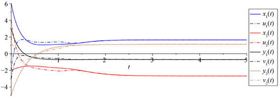
Figure 1. Curves of the $x_i\left(t\right)$, $y_j\left(t\right)$, $u_i\left(t\right)$, $v_j(\; k\; )$

图1. $x_i\left(t\right)$， $y_j\left(t\right)$， $u_i\left(t\right)$， $v_j\left(k\right)$ 的曲线

致谢

感谢审稿人对本文提出中肯的修改意见。特别感谢朱志强教授对本文写作过程的指导。