Fokker-Planck方程TVD有限体积方法

TVD Finite Volume Method for Fokker-Planck Equation

摘要: 我们研究一种求解时间分数阶Fokker-Planck方程TVD有限体积方法，其中对流项和扩散项分别使用TVD离散格式和中心差分离散格式，时间分数阶导数采用离散格式。数值实验结果表明，在较粗网格上求解对流占优问题时，我们的方法具有较好的优势。

Abstract: We study a TVD finite volume method for solving the time fractional Fokker-Planck equation, in which the TVD scheme and the central difference scheme are used to discretize the convection term and the diffusion term respectively, and L1 scheme is used to discretize the time fractional derivative. The numerical tests show that our method has advantages when it is used to solve convection dominated problems on coarse grids.

1. 研究问题

我们研究如下时间分数阶Fokker-Planck方程(FFPE)：

$\frac{{\partial }^{\alpha }w}{\partial t^{\alpha }}=\left(k_{\alpha }\frac{{\partial }^2}{\partial x^2}-\frac{\partial }{\partial x}f\left(x\right)\right)w\left(x,t\right),a\le x\le b,0\le t\le T,$ (1.1)

初始条件和边值条件为

$w\left(x,0\right)=\phi \left(x\right),a\le x\le b,w\left(a,t\right)=g_1\left(t\right),w\left(b,t\right)=g_2\left(t\right),0\le t\le T,$ (1.2)

其中 $\alpha \in \left(0,1\right)$， $k_{\alpha }$ 是正常数， $f\left(x\right),\phi \left(x\right),g_1\left(t\right),g_2\left(t\right)$ 是已经给定的函数，分数阶导数 ${\partial }^{\alpha }w/\partial t^{\alpha }$ 表示

$\alpha \left(0<\alpha <1\right)$ 阶Caputo分数阶导数： $\frac{{\partial }^{\alpha }w}{\partial t^{\alpha }}=\frac{1}{\text{Γ}\left(1-\alpha \right)}\frac{\partial }{\partial t}{\displaystyle {\int }_0^t\frac{\partial w\left(x,s\right)}{\partial t}\frac{\text{d}s}{{\left(t-s\right)}^{\alpha }}}$， $\Gamma \left(\alpha \right)$ 是Gamma函数。方程(1.1)

可以用来模拟受外力场作用下的反常扩散现象(参见文献 [1] )，此时 $k_{\alpha }$ 表示广义扩散系数， $f\left(x\right)$ 表示外力场。

我们研究求解(1.1)式的有限体积方法，其中对流项的离散使用TVD格式(TVD格式是由美国学者Harte提出的，它同时具有稳定、无振荡和高阶精度的数学特点，是较为先进的离散格式，参见文献 [2] )，空间扩散项的离散使用中心差分格式，时间分数阶导数离散采用L₁格式(参见文献 [3] )。

假设 $N,L$ 为正整数，我们取空间步长 $h=\left(b-a\right)/\left(N+1\right)$，时间步长 $\Delta t=T/L$。将区间 $\left[a,b\right]$ $N+1$ 等分，

分点为 $x_i=a+ih,i=0,1,2,\cdots ,N+1$。记 $x_{i+\frac{1}{2}}=\left(x_i+x_{i+1}\right)/2$，N个有限体积单元为 $\left[x_{i-\frac{1}{2}},x_{i+\frac{1}{2}}\right],i=0,1,2,\cdots ,N$ ；将 $\left[0,T\right]$ L等分，分点为 $t_k=k\Delta t,k=0,1,2,\cdots ,L$。为了便于描述，记 $f_{i+\frac{1}{2}}=f\left(x_{i+\frac{1}{2}}\right)$。

在方程(1.1)中取 $t=t_n\left(n=1,2,\cdots ,L\right)$，在有限体积单元 $\left[x_{i-\frac{1}{2}},x_{i+\frac{1}{2}}\right]$ 上对方程两边积分得

${\displaystyle {\int }_{x_{i-\frac{1}{2}}}^{x_{i+\frac{1}{2}}}{\frac{{\partial }^{\alpha }w}{\partial t^{\alpha }}|}_{t_n}}=k_{\alpha }\left[{\left(\frac{\partial w}{\partial x}\right)}_{i+\frac{1}{2}}^n-{\left(\frac{\partial w}{\partial x}\right)}_{i-\frac{1}{2}}^n\right]-\left[{\left(fw\right)}_{i+\frac{1}{2}}^n-{\left(fw\right)}_{i-\frac{1}{2}}^n\right],i=1,2,\cdots ,N.$ (1.3)

再对时间项用L₁格式离散，空间扩散项用中心差分格式离散，可得

$\begin{array}{l}\frac{h\Delta t^{-\alpha }}{\Gamma \left(2-\alpha \right)}\left(w_i^n-\underset{k=1}{\overset{n-1}{{\displaystyle \sum }}}\left(a_{n-k-1}-a_{n-k}\right)w_i^k-a_{n-1}{w}_i^0\right)\\ =\frac{k_{\alpha }}{h}\left(w_{i+1}^n-2w_i^n+w_{i-1}^n\right)-{\left(fw\right)}_{i+\frac{1}{2}}^n+{\left(fw\right)}_{i-\frac{1}{2}}^n,i=1,2,\cdots ,N\end{array}$ (1.4)

2. TVD格式离散对流项

对流项的TVD离散格式为

${\left(fw\right)}_{i+\frac{1}{2}}^n=f_{i+\frac{1}{2}}\left[w_i^n+\frac{1}{2}\psi \left(r_{i+\frac{1}{2}}^{+}\right)\left(w_{i+1}^n-w_i^n\right)\right],f_{i+\frac{1}{2}}>0$

${\left(fw\right)}_{i+\frac{1}{2}}^n=f_{i+\frac{1}{2}}\left[w_{i+1}^n-\frac{1}{2}\psi \left(r_{i+\frac{1}{2}}^{-}\right)\left(w_{i+1}^n-w_i^n\right)\right],f_{i+\frac{1}{2}}<0.$ (2.1)

其中

$r_{i+\frac{1}{2}}^{+}=\frac{w_i^n-w_{i-1}^n}{w_{i+1}^n-w_i^n},r_{i+\frac{1}{2}}^{-}=\frac{w_{i+2}^n-w_{i+1}^n}{w_{i+1}^n-w_i^n}.$ (2.2)

本篇文章中我们采用限制器Van Leer函数(参见 [4] )： $\psi \left(r\right)=\frac{r+\left|r\right|}{1+\left|r\right|}$。

对于一维Fokker-Planck方程，将(2.1) (2.2)式代入(1.1)式，经过运算以及整理可得离散格式为，对 $i=1,2,\cdots ,N$，

$F_i\left(w_{i-1}^n,w_i^n,w_{i+1}^n\right)+G_i\left(w_{i-1}^n,w_i^n,w_{i+1}^n\right)=\frac{h\Delta t^{-\alpha }}{\Gamma \left(2-\alpha \right)}\left({\displaystyle {\sum }_{k=1}^{n-1}\left(a_{n-k-1}-a_{n-k}\right)w_i^k}-a_{n-1}{w}_i^0\right).$ (2.3)

其中

$\begin{array}{c}{F}_i\left(w_{i-1}^n,w_i^n,w_{i+1}^n\right)=\frac{1}{2}{f}_{i+\frac{1}{2}}\left[\beta \psi \left(r_{i+\frac{1}{2}}^{+}\right)-\bar{\beta }\psi \left(r_{i+\frac{1}{2}}^{-}\right)\right]\left(w_{i+1}^n-w_i^n\right)\\ -\frac{1}{2}{f}_{i-\frac{1}{2}}\left[\beta \psi \left(r_{i-\frac{1}{2}}^{+}\right)-\bar{\beta }\psi \left(r_{i-\frac{1}{2}}^{-}\right)\right]\left(w_i^n-w_{i-1}^n\right)\end{array}$ (2.4)

$\begin{array}{c}{G}_i\left(w_{i-1}^n,w_i^n,w_{i+1}^n\right)=-\left[\max \left(f_{i-\frac{1}{2}},0\right)+\frac{k_{\alpha }}{h}\right]w_{i-1}^n-\left[\max \left(-f_{i+\frac{1}{2}},0\right)+\frac{k_{\alpha }}{h}\right]w_{i+1}^n\\ +\left[\max \left(f_{i-\frac{1}{2}},0\right)+\max \left(-f_{i+\frac{1}{2}},0\right)+\left(f_{i+\frac{1}{2}}-f_{i-\frac{1}{2}}\right)+\frac{2k_{\alpha }}{h}+\frac{h\Delta t^{-\alpha }}{\Gamma \left(2-\alpha \right)}\right]w_i^n\end{array}$ (2.5)

在(2.4)式中，为了简便，定义了补函数，即 $\bar{\beta }\equiv 1-\beta$。使用迭代法求解离散问题(2.3)，迭代过程中 $F_i\left(w_{i-1}^n,w_i^n,w_{i+1}^n\right)$ 中的 $w^n$ 使用旧近似值， $G_i\left(w_{i-1}^n,w_i^n,w_{i+1}^n\right)$ 中的 $w^n$ 使用新近似值，每一步迭代中线性问题求解使用稳定双共轭梯度法(参见 [5] )。

3. 数值实验及结论

算例1考虑以下Fokker-Planck方程

$\frac{{\partial }^{\alpha }w}{\partial t^{\alpha }}=\left(k_{\alpha }\frac{{\partial }^2}{\partial x^2}-\frac{\partial }{\partial x}f\left(x\right)\right)w\left(x,t\right)+G\left(x,t\right),0\le x\le 1,0\le t\le 1,$

其中 $k_{\alpha }=1$, $G\left(x,t\right)=0$, $f\left(x\right)=\{\begin{array}{l}100,x>0.5\\ 50,x\le 0.5\end{array}$。

初始值和边界值分别为

$w\left(x,0\right)=0,g_1\left(t\right)=t^2\cos \left(2\pi \right),g_2\left(t\right)=t^2\cos \left(-2\pi \right).$

图1展示的是TVD有限体积方法和中心差分格式有限体积法求解效果图，其中 $L=100,\alpha =0.2$，从实

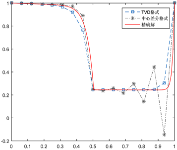
Figure 1. Comparison of solving effects of N = 15 (left) and N = 25 (right)

图1. N = 15求解效果对比(左)；N = 25求解效果对比(右)

验结果可以看出在较粗网格上求解对流占优问题时，中心差分格式会产生振荡，而TVD格式始终保持稳定。