1. 引言
非线性演化方程的精确解在非线性科学领域,特别是在光学、流体、玻色–爱因斯坦凝聚体和等离子体等领域具有重要的意义 [1] - [6],它可以为我们提供更多的物理信息,加深人们对一些非线性波动现象的理解,从而得到广泛的应用。怪波 [7]、孤立波 [8] 和lump波 [9] [10] 等都属于非线性波。
考虑(2 + 1)维Hirota-Satsuma-Ito (HSI)方程 [11]
(1)
其中
表示空间坐标,t表示时间,u是关于
的函数,
是任意常数。目前一些学者已经对HSI方程进行了研究 [11] [12] [13],而对于HSI方程的态转换在很大程度上仍未被探索。在本文中,我们利用双线性方法求得HSI方程的呼吸波解,进而通过分析特征线的性质找到呼吸波发生态转换的条件,并研究这些转换波的动力学行为。
本文的结构安排如下:第2部分给出了HSI方程的呼吸波解以及呼吸波发生态转换的条件。第3部分介绍了三类转换波的类型。第4部分给出了本文的一些结论。
2. 呼吸波解和态转换条件
通过变量变换 [14]
(2)
可以得到方程(1)的双线性形式,即
(3)
其中双线性算子D的定义如下 [15]:
(4)
首先利用二阶孤子解来求呼吸波解,下面给出
:
(5)
设
,其中
(6)
是一些自由参量,我们对这些参量进行复数化,即:
(7)
*代表共轭,
都是实常数。将式(6)和(7)代入到式(5)中,可以得到
(8)
其中
(9)
(10)
把式(8)代入到式(2)里,就得到了HSI方程的一阶呼吸波解,表示为:
(11)
呼吸波解的特征线方程可以求得如下:
(12)
通过分析特征线的性质,可以发现当特征线方程满足以下条件时,
(13)
即两条特征线平行时,呼吸波就发生了态转换。下面我们详细分析这些转换波的动力学行为。
3. 转换波的类型
3.1. W型、M型
根据转换条件(13),我们来研究转换非线性波的动力学特征,并且在计算模拟过程中发现波数
和
对转换波的类型有很大的影响。首先考虑一种情况,
。这时呼吸波在转换条件下就变成了W型和M型波,如图1所示。从图中可以看出,随着时间的推移,转换波的波形从M型变成了W型,紧接着又从W型变回了M型。经过分析这组转换波随时间变化的动态图,发现在这组参数下,转换波的形状在M型和W型之间交替出现。通过观察这三个时刻的密度图,可以清晰的看到,随时间的推移,除了转换波的形状发生改变外,它的位置也发生了变化,但是波在运动过程中斜率没发生变化,同时可以观察到M型波的宽度大于W型波。
通过图2可以直观地看出这三个时刻的转换波的横截面的形状,其中两个M型波除了位置不同外,它们的振幅和宽度都几乎相同,W型波的振幅相对于这两个M型波来说更大一些,而波的宽度更窄一些。M型波有两个波峰和一个波谷,W型波有一个波峰和两个波谷。
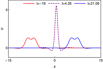
Figure 2. Sectional view of three moments
图2. 三个时刻的截面图
3.2. 振荡W型、振荡M型
对比本章节中的第一部分W型波和M型波对应的参数,现在保持
的值不变,增大
的值,取
,此时的转换波就变成了带有振荡行为的W型和M型波,即振荡W型波和振荡M型波,如图3所示。与图2中的转换波相比,此时的振荡W型和M型波的波峰和波谷都增加了许多。通过三维图和密度图都可以看出,随着时间的变化,振荡型波在平面上移动,但是斜率保持不变。
通过图4,可以看到振荡型波的截面图的形状是在振荡W型和振荡M型之间交替出现的,并且能明显看出波峰和波谷的数量比之前的W型和M型波增多了,此时两个振荡W型波的振幅明显大于振荡M型波,而且这两个振荡W型波的形状几乎完全相同,只有位置发生了变化。
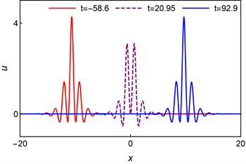
Figure 4. Sectional view of three moments
图4. 三个时刻的截面图
3.3. 准周期型
相反地,现在保持
的值不变,减小
的值,我们取
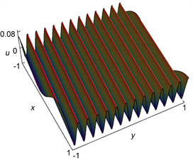
,这时候转换波的振荡频率大大增加了,并表现出了一定的周期行为,我们把这种有周期行为的波叫做准周期波,图5给出了两个时刻的准周期波,它们可以看成是由一系列的W型或者M型波元构成的波。从三维图中几乎看不出两个波的区别,但是从密度图可以看出,在y轴方向上,第一个时刻的波在y = 1附近密度图上呈现出橘色,而第二个时刻的波在y = 1附近,密度图呈现红色,所以发现这两个时刻的波的高度是不同的,二者存在一定的区别。
 (a)
(a)  (b)
(b) 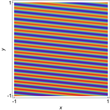 (c)
(c) 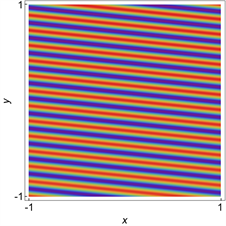 (d)
(d)
Figure 5. Converted waves at different times: (a) t = 37; (b) t = 45; (c) t = 92.9; (c) and (d) are the corresponding density maps respectively
图5. 不同时刻的转换波:(a) t = 37;(b) t = 45;(c)和(d)分别是对应的密度图
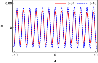
Figure 6. Sectional view of two moments
图6. 两个时刻的截面图
我们再来观察y = 0时的准周期波的截面图,此时两个波的不同之处显而易见,当t = 37时,准周期波的振幅在x轴方向上从左到右逐渐减小,而到了t = 45时刻,准周期波的振幅从左到右逐渐增大。我们之所以称它们为准周期波,是因为这些波只是表现出了一定的周期态,但并不是完完全全的周期波。
4. 结论
本文研究了2 + 1维HSI方程,在特定的条件下,可将HSI方程的呼吸波转换成其他类型的非线性波,比如(振荡-)W型和(振荡-)M型波(见图1~4),准周期波(见图5、图6)。我们发现这些转换波在运动的过程中,形状都发生了改变,而斜率保持不变。此外,波数
和
影响着转换波的类型,固定
的值同时增大
的值,转换波表现出一定的振荡行为,固定
的值同时减小
的值,转换波表现出一定的周期态,从而发现
值的增大会使得转换波的频率增加。研究结果丰富了2 + 1维非线性波的动力学行为。