具有执行器饱和的广义随机系统的滑模自适应控制

Sliding Mode Adaptive Control for Singular Stochastic Systems with Time-Delay and Uncertainty

摘要: 本文主要研究了具有时滞不确定性的广义随机系统的滑模自适应控制问题。首先设计了适合可行的积分型滑模面函数，进一步求得等效控制器，从而得到了闭环系统，利用LMI和李雅普诺夫函数理论，得到闭环系统带有H∞扰动衰减水平的容许性；设计一种新的自适应滑模控制率，保证了滑模面的有限时间可达性。最后，用一个算例仿真证明了本文所提方法的有效性。

Abstract: In this paper, the problem of adaptive sliding mode control for singular stochastic systems with delay uncertainties is studied. Firstly, a suitable and feasible integral sliding mode surface function is designed, and the equivalent controller is obtained to get the closed-loop system. By using LMI and Lyapunov function theory, the permissibility of the closed-loop system with disturbance attenuation level is obtained. A new adaptive sliding mode control rate is designed to ensure the finite time accessibility of the sliding mode surface. Finally, a numerical example is given to demonstrate the effectiveness of the proposed method.

1. 引言

奇异随机系统是具有随机扰动的奇异动力系统，它能更真实合理地描述实际模型的复杂性。Gibbs [1] 首先提出了随机微分。目前，控制奇异随机系统的研究还处于初级阶段，因此对奇异随机系统的研究比以往困难得多，特别是对控制奇异随机系统的研究。专家学者对SSS的稳定性和控制设计进行了进一步的研究，这也适用于有较高要求的系统。因此，Liu [2] 研究了SSS的积分滑模自适应控制。基于马尔可夫跳变参数，Xia [3] 研究了不确定时滞SSS的鲁棒滤波器设计问题。Lu [4] 基于非线性时延SSS进行了研究，研究了时延相关的耗散滤波。此外，Ma [5] 还研究了不确定离散时滞SSS的鲁棒稳定性和镇定性。

执行器饱和系统的存在会降低系统的动态性能，使闭环系统处于不稳定状态。到目前为止，学者们总结出了许多有效的饱和处理方法，常用的方法有凸组合法、扇形面积法和饱和法。2003年，曹艳艳 [6] 等人对受饱和影响的离散时间线性系统进行了研究，巧妙地利用凸组合法处理饱和问题，给出了系统的稳定性判据。在文献 [7] 中基于饱和线性状态反馈，利用凸组合方法研究了奇异线性系统的吸引域估计问题。Ma Y. M.和Chen Q. [8] [9] 等人利用凸组合方法估计了离散时间线性饱和系统的吸引域，分析了系统的稳定性。李彦龙、史涛等人利用凸组合法处理饱和问题，估计了连续线性饱和系统的吸引域。因此，文献 [10] [11] 中结果的保守性明显降低。Daniel W. C. [12] 等人研究了具有非线性扰动和致动器饱和的奇异系统的容错控制问题。此外，在文献 [13] 中给出了致动器饱和时滞系统吸引域的估计方法和系统稳定性条件。在积分不等式的基础上，Fu L., Ma Y. C. [14] 给出了具有驱动器饱和的非线性奇异时滞系统耗散性能的一个充分条件。他们利用线性矩阵不等式(LMI)合成了无源状态反馈控制器。此外，文献 [15] [16] 研究了具有执行器饱和和不确定奇异时滞系统的离散切换奇异时滞系统的有限时间 $H_{\infty }$ 控制。R. Sakthivel [17] 等人研究了中立系统针对执行器饱和和非线性故障的有限时间容错控制。

滑模控制，又称变结构控制，实际上是非线性控制的一种特殊的控制方法。它对外界干扰具有较强的鲁棒性，并利用滑动面和等效控制来处理不确定系统和非线性系统。滑模可设计，且不受物体参数和摄动的影响，因此滑模具有响应速度快、适应性强等优点。SMC打破了传统控制设计的性能限制，使其能够自我保持性能优于一般固定结构。因此，平衡问题在文献 [18] 中解决了动态和静态性能指标之间存在的问题。通过学者在 [19] 中的研究和探索，SMC逐渐成为一个相对独立的分支。适用于离散系统、连续系统、集中参数系统和分布参数系统 [20] [21]。目前，变结构控制理论已经进入了一个新的研究阶段，对其研究对象进行的探讨已经扩展到许多复杂系统，包括离散系统 [22]，分布式函数系统 [23] [24]，广义系统 [25]，时滞系统 [26]，非线性大规模系统 [27]。近年来，SMC主要研究滑模面设计、抖振问题、自适应滑模变结构控制等课题，其中抖振问题是非常重要的角色。学者们给出的许多不同的解决方案可以概括为两点。一个是研究滑模运动，从滑模运动中设计避免或减少抖振的方法，例如时变滑动面 [28] [29] [30]。二是研究变结构设计旨在使系统运动到达跳跃面附近的控制器不会经历它们结构的突然变化。虽然对SMC的研究已经取得了一定的进展取得了一些成绩，还可以从多方面进行研究。例如，梳理SMC再加上其他的控制理论，或者像这样的一些话题，将成为未来的发展方向研究。

在奇异系统中，关于致动器饱和的求解已经在许多文献中取得了大量的研究成果，Ma Y.C., Liu Y.F., Liu N. [31] 报道了奇异马尔科夫跳变系统的可靠有限时间 $H_{\infty }$ 控制。M. Kchaou [32] 和Palanisamy S. [33] 等分别讨论了执行器饱和的广义模糊系统的滑模容错控制问题。但是如何解决SMC系统中执行器饱和问题的研究却很少，且此类系统满足均方渐近可容许性能的充分条件是什么？这也是本文的研究目的。因此，本文对于研究具有致动器饱和的奇异随机系统的滑模自适应控制具有重要意义。难点在于如何处理有限时间可达条件下的执行器饱和问题。

在此基础上，本文的主要贡献如下：研究了滑模自适应控制中致动器饱和的奇异随机系统，为滑模控制中致动器饱和的问题提供了一种可靠的解决方案。利用特殊观测器设计并构造了一种新型滑模面，利用线性矩阵不等式(LMI)给出了闭环系统，并给出了SMDs稳定的充分条件。提出了一种混合自适应控制器来保证滑模面在有限时间内的可达性。最后，通过实例仿真验证了所提理论的有效性。

符号说明： $\left(\Omega ,F,L\right)$ 代表完整的概率空间；“*”代表对称矩阵中的对称元素；“T”代表标量或矩阵的转置； $sym\left\{A\right\}$ 代表 $A+A^{\text{T}}$ ； $\epsilon$ 代表标量或者矩阵的期望； $\Vert \cdot \Vert$ 代表标量或矩阵的范数； $\sup \{\cdot \}$ 代表矩阵的上界； $\text{inf}\{\cdot \}$ 代表矩阵的下界。

2. 系统模型

考虑如下广义随机系统：

$\{\begin{array}{l}E\text{d}x\left(t\right)=\left[\left(A+\Delta A\left(t\right)\right)x\left(t\right)+Bsat\left(u\left(t\right)\right)+f\left(x,t\right)+Dv\left(t\right)\right]\text{d}t+Fx\left(t\right)\text{d}\omega \left(t\right)，\\ y\left(t\right)=Cx\left(t\right)，\\ x\left(0\right)=x_0\end{array}$ (1)

其中， $x\left(t\right)\in R^n$ 表示状态变量， $u\left(t\right)\in R^m$ 表示控制输入信号， $y\left(t\right)\in R^p$ 表示测量输出信号， $f\left(x,t\right)$ 是非线性扰动输入函数， $v\left(t\right)\in R^l$ 是外部扰动， $\omega \left(t\right)$ 为定义在概率空间 $\left(\Omega ,F,L\right)$ 上的标准的一维维纳过程且满足 $E\left\{\text{d}\omega \left(t\right)\right\}=0$， $x_0$ 为系统初始值， $A,B,C,D,F$ 为具有适当维数的实常数矩阵。B为列满秩矩阵， $E\in R^{n\times n}$ 为奇异矩阵，满足 $rank\left(E\right)=r\le n$ 且 $rank\left(E\right)=rank\left(E,B_{\omega }\right)$。

饱和函数 $sat\left(u\left(t\right)\right)$ 的定义如下

$sat\left(u\left(t\right)\right)={\left[sat\left(u_1\left(t\right)\right),sat\left(u_2\left(t\right)\right),\cdots ,sat\left(u_p\left(t\right)\right)\right]}^{\text{T}}$,

为了不失一般性

$sat\left(u\left(t\right)\right)=sat\left(u_i\left(t\right)\right)\cdot \min \left\{1,\left|u_i\left(t\right)\right|\right\}=\{\begin{array}{l}1,u_j\left(t\right)>1;\\ u_j\left(t\right),-1<u_j\left(t\right)<1;\\ -1,u_j\left(t\right)<-1\end{array}$ (2)

其中 $j=1,2,\cdots ,q$。

对于系统(1)给出如下假设：

假设2.1： $\Delta A\left(t\right)$ 为范数有界的不确定参数矩阵，并且有可表示为

$\Delta A\left(t\right)=MJ\left(t\right)N$

其中， $M,N$ 都是适当维数的实常数矩阵， $J\left(t\right)$ 是未知矩阵且满足 $J^{\text{T}}\left(t\right)J\left(t\right)\le I$。

假设2.2：对于 $\forall x_1,x_{\text{2}}，f\left(x,t\right)$ 满足

$\Vert f\left(x_1,t\right)-f\left(x_2,t\right)\Vert \le \rho \Vert x_1-x_2\Vert$

其中 $\rho >0$ 是未知的。

假设2.3：系统(1)是正则且无脉冲的。

引理2.1 (Schur补引理)：对给定的对称矩阵 $S=\left[\begin{array}{cc}{S}_{11}& S_{\text{12}}\\ S_{12}^{\text{T}}& S_{\text{22}}\end{array}\right]$，其中 $S\in R^{n\times n}$， $S_{\text{11}}\in R^{r\times r}$ 维的。以下3个条件是等价的：

1) $S<0;$

2) $S_{\text{11}}<0,S_{\text{22}}-S_{12}^{\text{T}}{S}_{11}^{-1}{S}_{\text{12}}<0;$

3) $S_{\text{22}}<0,S_{\text{11}}-S_{\text{12}}{S}_{22}^{-1}{S}_{12}^{\text{T}}<0.$

引理2.2：设 $X,Y$ 和 $J\left(t\right)$ 是具有适当维数的实矩阵。 $\epsilon >0$ 是任意给定的常数，则有

$sym\left\{XJ\left(t\right)Y\right\}\le {\epsilon }^{-1}X{X}^{\text{T}}+\epsilon Y^{\text{T}}Y$

定义1：如果系统(1)是正则、无脉冲且稳定的。则称系统(1)是容许的。

定义2：如果满足如下两个条件：

a) 当 $v\left(t\right)=0$ 时，系统(4)是容许的；

b) 在零初始条件下，在非零外部扰动 $v\left(t\right)\in L_2\left[0,\infty \right)$ 和给定的衰减水平 $\gamma >0$ 下，保持以下性能指标：

${\displaystyle {\int }_{\text{0}}^{\infty }{y}^{\text{T}}\left(t\right)y\left(t\right)\text{d}t}\le {\gamma }^2{\displaystyle {\int }_{\text{0}}^{\infty }{v}^{\text{T}}\left(t\right)v\left(t\right)\text{d}t}$

称闭环系统(4)在 $H_{\infty }$ 扰动衰减水平 $\gamma$ 下是均方渐近容许。

3. 主要结果

3.1. 非脆弱观测器

$\{\begin{array}{l}E\text{d}x\left(t\right)=[A\hat{x}\left(t\right)+Bsat\left(u\left(t\right)\right)+f\left(\hat{x},t\right)+\left(L+\Delta L\left(t\right)\right)\left(y\left(t\right)-Cx\left(t\right)\right)]\text{d}t\\ \hat{y}\left(t\right)=C\hat{x}\left(t\right)，\\ \hat{x}\left(0\right)={\hat{x}}_0\end{array}$ (3)

其中： $\hat{x}\left(t\right)$ 表示状态变量 $x\left(t\right)$ 的估计， $\hat{y}\left(t\right)$ 表示测量输出信号 $y\left(t\right)$ 的估计， $L\in R^{n\times p}$ 是待定的观测器增益。 $\Delta L\left(t\right)$ 满足 $\Vert \Delta L\left(t\right)\Vert \le \delta$，其中标量 $\delta >0$。

定义误差系统为 $e\left(t\right)=x\left(t\right)-\hat{x}\left(t\right)$，由等式(1)和(3)得误差系统如下

$\{\begin{array}{l}E\text{d}e\left(t\right)=\{\left[A-\left(L+\Delta L\left(t\right)\right)C\right]e\left(t\right)+\Delta Ax\left(t\right)+f\left(x,t\right)-f\left(\hat{x},t\right)+Dv\left(t\right)\}\text{d}t+Fx\left(t\right)\text{d}\omega \left(t\right)\\ y_e\left(t\right)=Ce\left(t\right)，\end{array}$ (4)

其中 $y_e\left(t\right)$ 代表误差系统的输出变量。

在此，介绍一下 $H_{\infty }$ 性能指标：

$\epsilon \left\{\underset{0\ne v(t)\in L_2\left[0,\infty \right)}{\sup }\frac{{\Vert y_e\left(t\right)\Vert }_2}{{\Vert v\left(t\right)\Vert }_2}\right\}<\gamma$. (5)

3.2. 设计滑模面及滑模控制

在本节中，给出一个积分滑模面函数为

$s\left(t\right)=G\left[Ee\left(t\right)-Ee\left(0\right)\right]+G\left[E\hat{x}\left(t\right)-E\hat{x}\left(0\right)\right]-{\displaystyle {\int }_0^{t}G\left(A+BK\right)}x\left(\tau \right)\text{d}\tau$ (6)

其中K为控制器增益。矩阵 $G\in R^{m\times n}$ 是已知的常数矩阵且满足GB是非奇异的。

注：滑模面函数(6)的可行性具体请参照文献 [2]。

接下来，使滑模面 $s\left(t\right)=0$ 在给定时间T内可达，使得系统的状态轨迹在有限时间内能够驱动到滑模面上，且在随后的时间保持在滑模面上。

$\begin{array}{l}\text{d}s\left(t\right)=GE\text{d}e\left(t\right)+GE\text{d}\hat{x}\left(t\right)-G\left(A+BK\right)\hat{x}\left(t\right)\text{d}t\\ =Ls\left(t\right)\text{d}t+GFx\left(t\right)\text{d}\omega \left(t\right)\end{array}$ (7)

其中

$Ls\left(t\right)=G\left[Ae\left(t\right)+\Delta A\left(t\right)x\left(t\right)-BK\hat{x}\left(t\right)+Bsat\left(u\left(t\right)\right)+f\left(x,t\right)+Dv\left(t\right)\right]$

令 $Ls\left(t\right)=0$，可得

$sa{t}_{eq}\left(u\left(t\right)\right)=K\hat{x}\left(t\right)-{\left(GB\right)}^{-1}GAe\left(t\right)-{\left(GB\right)}^{-1}G\Delta A\left(t\right)x\left(t\right)-{\left(GB\right)}^{-1}Gf\left(x,t\right)-{\left(GB\right)}^{-1}GDv\left(t\right)h$ (8)

将等式(8)分别带入等式(1)和(4)，得闭环系统：

$E\text{d}x\left(t\right)=\{\left[\left(A+BK\right)+B_G\Delta A\left(t\right)\right]x\left(t\right)+\left(B_{G}A+BK\right)e\left(t\right)+B_{G}f\left(x,t\right)+B_{G}v\left(t\right)\}\text{d}t+Fx\left(t\right)\text{d}\omega \left(t\right)$ (9)

$E\text{d}e\left(t\right)=\left\{\left[A-\left(L+\Delta L\left(t\right)\right)C\right]e\left(t\right)+\Delta Ax\left(t\right)+f\left(x,t\right)-f\left(\hat{x},t\right)+Dv\left(t\right)\right\}\text{d}t+Fx\left(t\right)\text{d}\omega \left(t\right)$ (10)

其中： $B_G=I-B\left(GB\right){}^{-1}G$， $G_B=B\left(GB\right){}^{-1}G$。

接下来，称等式(9)和(10)为闭环系统的SMDs。

4. 性能分析

4.1. 有限时间可达性

本节通过设计合适的自适应控制器，保证了滑模相位的有限时间可达性。该方法不同于一般的可达性证明，在一定程度上可以减缓滑动面附近滑模函数的抖振现象。下面是一个自适应滑模控制器

$sat\left(u\left(t\right)\right)=\{\begin{array}{l}{u}_1,u\left(t\right)>1;\\ u_2,-0<u\left(t\right)<1;\\ u_3,u\left(t\right)<-1\end{array}$ (11)

其中

$u_{\text{1}}\left(t\right)=\Vert K\Vert \Vert \hat{x}\left(t\right)\Vert -\Vert {\hat{l}}_1\left(t\right)\Vert \Vert y\left(t\right)\Vert -\Vert {\hat{l}}_{\text{2}}\left(t\right)\Vert \Vert \hat{y}\left(t\right)\Vert -\Vert {\hat{l}}_3\left(t\right)\Vert -\sigma$,

$u_{\text{2}}\left(t\right)=K\hat{x}\left(t\right)-{\left(GB\right)}^{-1}\left({\hat{l}}_1\left(t\right)\Vert y\left(t\right)\Vert +{\hat{l}}_{\text{2}}\left(t\right)\Vert \hat{y}\left(t\right)\Vert +{\hat{l}}_3\left(t\right)+\rho \right)\mathrm{sgn}\left(s\left(t\right)\right)$,

$u_{\text{3}}\left(t\right)=-\Vert K\Vert \Vert \hat{x}\left(t\right)\Vert +\Vert {\hat{l}}_1\left(t\right)\Vert \Vert y\left(t\right)\Vert +\Vert {\hat{l}}_{\text{2}}\left(t\right)\Vert \Vert \hat{y}\left(t\right)\Vert +\Vert {\hat{l}}_3\left(t\right)\Vert +\sigma$

其中： $l_i>0\left(i=1,2\right)$ 是上界不可知未知标量。令 ${\hat{l}}_1\left(t\right)$ 和 ${\hat{l}}_{\text{2}}\left(t\right)$ 分别为误差 ${\tilde{l}}_1\left(t\right)={\hat{l}}_1\left(t\right)-l_1$ 和 ${\tilde{l}}_{\text{2}}\left(t\right)={\hat{l}}_{\text{2}}\left(t\right)-l_{\text{2}}$ 的估计值，并且， ${\tilde{l}}_{\text{3}}\left(t\right)={\hat{l}}_{\text{3}}\left(t\right)-l_{\text{3}}$。在此，更新率设为 ${\stackrel{\dot{}}{\hat{l}}}_1\left(t\right)=l_1\Vert y\left(t\right)\Vert \Vert s\left(t\right)\Vert$ 和 ${\stackrel{\dot{}}{\hat{l}}}_{\text{2}}\left(t\right)=l_1\Vert y\left(t\right)\Vert \Vert s\left(t\right)\Vert$， ${\stackrel{\dot{}}{\hat{l}}}_3\left(t\right)=l_3\Vert s\left(t\right)\Vert$。 $l_i>0\left(i=1,2,\text{3}\right)$ 是设计者选择的自适应增益的正标量， $\rho$ 是正标量。

在本节证明中，应用一个不等式

$\begin{array}{c}\psi =\Vert GA\left(t\right)\Vert \Vert e\left(t\right)\Vert +\Vert G\Delta A\left(t\right)\Vert \Vert x\left(t\right)\Vert +\Vert G\Vert \Vert f\left(x,t\right)\Vert +\Vert GD\Vert \Vert v\left(t\right)\Vert \\ \le l_1\Vert y\left(t\right)\Vert +l_2\Vert \hat{y}\left(t\right)\Vert +l_3\end{array}$ (12)

定理1：若滑模自适应控制率设计为(11)，则可以保证滑模面(6)的有限时间可达性。

证明：选择如下李雅普诺夫函数

$\bar{V}\left(t,s\left(t\right)\right)=\frac{s^{\text{T}}\left(t\right)s\left(t\right)}{\Vert s\left(t\right)\Vert }+\frac{{\tilde{l}}_1^2\left(t\right)}{2l_1}+\frac{{\tilde{l}}_2^2\left(t\right)}{2l_2}+\frac{{\tilde{l}}_3^2\left(t\right)}{2l_3}$

求得 $\bar{V}\left(t,s\left(t\right)\right)$ 的随机微分，有

$\begin{array}{c}\text{d}\bar{V}\left(t,s\left(t\right)\right)=\frac{s^{\text{T}}\left(t\right)}{\Vert s\left(t\right)\Vert }\text{d}s\left(t\right)+\frac{{\tilde{l}}_1\left(t\right){\stackrel{\dot{}}{\tilde{l}}}_1\left(t\right)\text{d}t}{l_1}+\frac{{\tilde{l}}_2\left(t\right){\stackrel{\dot{}}{\tilde{l}}}_2\left(t\right)\text{d}t}{l_2}+\frac{{\tilde{l}}_3\left(t\right){\stackrel{\dot{}}{\tilde{l}}}_3\left(t\right)\text{d}t}{l_3}\\ =L\bar{V}\left(t,s\left(t\right)\right)\text{d}t+\frac{s^{\text{T}}\left(t\right)}{\Vert s\left(t\right)\Vert }GFx\left(t\right)\text{d}\omega (\; t\; )\end{array}$

其中

$\begin{array}{c}L\bar{V}\left(t,s\left(t\right)\right)=\frac{s^{\text{T}}\left(t\right)}{\Vert s\left(t\right)\Vert }\left\{GAe\left(t\right)+G\Delta A\left(t\right)x\left(t\right)-GBK\hat{x}\left(t\right)+GBsat\left(u\left(t\right)\right)+Gf\left(x,t\right)+GDv\left(t\right)\right\}\\ +\frac{{\tilde{l}}_1\left(t\right){\stackrel{\dot{}}{\tilde{l}}}_1\left(t\right)}{l_1}+\frac{{\tilde{l}}_2\left(t\right){\stackrel{\dot{}}{\tilde{l}}}_2\left(t\right)}{l_2}+\frac{{\tilde{l}}_3\left(t\right){\stackrel{\dot{}}{\tilde{l}}}_3\left(t\right)}{l_3}\end{array}$ (13)

因为 $l_i\left(t\right)\left(i=1,2,3\right)$ 和 ${\hat{l}}_i\left(t\right)\left(i=1,2,3\right)$ 的关系如下

${\tilde{l}}_1\left(t\right)={\hat{l}}_1\left(t\right)-l_1,{\tilde{l}}_{\text{2}}\left(t\right)={\hat{l}}_{\text{2}}\left(t\right)-l_{\text{2}},{\tilde{l}}_{\text{3}}\left(t\right)={\hat{l}}_{\text{3}}\left(t\right)-l_{\text{3}}$ (14)

并且

${\stackrel{\dot{}}{\tilde{l}}}_1\left(t\right)={\stackrel{\dot{}}{\hat{l}}}_1\left(t\right),{\stackrel{\dot{}}{\tilde{l}}}_{\text{2}}\left(t\right)={\stackrel{\dot{}}{\hat{l}}}_{\text{2}}\left(t\right),{\stackrel{\dot{}}{\tilde{l}}}_{\text{3}}\left(t\right)={\stackrel{\dot{}}{\hat{l}}}_{\text{3}}\left(t\right)$ (15)

利用等式(14)和(15)，将等式(11)带入(13)，并结合不等式(12)，有

1) 当 $u\left(t\right)>1$ 时，

$\begin{array}{l}L\bar{V}\left(t,s\left(t\right)\right)=\frac{s^{\text{T}}\left(t\right)}{\Vert s\left(t\right)\Vert }\{GAe\left(t\right)+G\Delta A\left(t\right)x\left(t\right)-GBK\hat{x}{\left(t\right)}_{}^{{}^{}}\\ +GB\left(\Vert K\Vert \Vert \hat{x}\left(t\right)\Vert -\Vert {\hat{l}}_1\left(t\right)\Vert \Vert y\left(t\right)\Vert -\Vert {\hat{l}}_2\left(t\right)\Vert \Vert \hat{y}\left(t\right)\Vert -\Vert {\hat{l}}_3\left(t\right)\Vert -\sigma \right)+Gf\left(x,t\right)+GDv\left(t\right)\}\\ +\frac{{\tilde{l}}_1\left(t\right){\stackrel{\dot{}}{\tilde{l}}}_1\left(t\right)}{l_1}+\frac{{\tilde{l}}_2\left(t\right){\stackrel{\dot{}}{\tilde{l}}}_2\left(t\right)}{l_2}+\frac{{\tilde{l}}_3\left(t\right){\stackrel{\dot{}}{\tilde{l}}}_3\left(t\right)}{l_3}\end{array}$

$\begin{array}{l}\le \left[\Vert s\left(t\right)\Vert \left(l_1\Vert y\left(t\right)\Vert +\Vert l_2\Vert \Vert \hat{y}\left(t\right)\Vert +l_3\right)-\Vert l_1\left(t\right)\Vert \Vert y\left(t\right)\Vert -\Vert l_2\left(t\right)\Vert \Vert \hat{y}\left(t\right)\Vert -\Vert l_3\Vert -\sigma \right]\\ +\frac{{\tilde{l}}_1\left(t\right){\stackrel{\dot{}}{\tilde{l}}}_1\left(t\right)}{l_1}+\frac{{\tilde{l}}_2\left(t\right){\stackrel{\dot{}}{\tilde{l}}}_2\left(t\right)}{l_2}+\frac{{\tilde{l}}_3\left(t\right){\stackrel{\dot{}}{\tilde{l}}}_3\left(t\right)}{l_3}\\ =-\sigma <0\end{array}$ (16a)

2) 当 $-\text{1}<u\left(t\right)<1$ 时，

$\begin{array}{c}L\bar{V}\left(t,s\left(t\right)\right)\le \Vert s\left(t\right)\Vert [\left(l_1\Vert y\left(t\right)\Vert +\Vert l_2\Vert \Vert \hat{y}\left(t\right)\Vert +l_3\right)-{\hat{l}}_1\left(t\right)\Vert y\left(t\right)\Vert -{\hat{l}}_2\left(t\right)\Vert \hat{y}\left(t\right)\Vert -{\hat{l}}_3\left(t\right)-\rho ]\\ +\frac{{\tilde{l}}_1\left(t\right){\stackrel{\dot{}}{\tilde{l}}}_1\left(t\right)}{l_1}+\frac{{\tilde{l}}_2\left(t\right){\stackrel{\dot{}}{\tilde{l}}}_2\left(t\right)}{l_2}+\frac{{\tilde{l}}_3\left(t\right){\stackrel{\dot{}}{\tilde{l}}}_3\left(t\right)}{l_3}\end{array}$

由等式(14)和(15)得

$\begin{array}{l}L\bar{V}\left(t,s\left(t\right)\right)\le \Vert s\left(t\right)\Vert [l_3-{\tilde{l}}_1\left(t\right)\Vert y\left(t\right)\Vert -{\tilde{l}}_2\left(t\right)\Vert \hat{y}\left(t\right)\Vert -{\hat{l}}_3\left(t\right)-\rho ]\\ +\frac{{\tilde{l}}_1\left(t\right)l_{\text{1}}\Vert y\left(t\right)\Vert \Vert s\left(t\right)\Vert }{l_1}+\frac{{\tilde{l}}_2\left(t\right)l_2\Vert y\left(t\right)\Vert \Vert s\left(t\right)\Vert }{l_2}+\frac{{\tilde{l}}_3\left(t\right)l_3\Vert s\left(t\right)\Vert }{l_3}\\ =-\rho <0\end{array}$ (16b)

3) 当 $u\left(t\right)<-1$ 时，

$\begin{array}{c}L\bar{V}\left(t,s\left(t\right)\right)=\frac{s^{\text{T}}\left(t\right)}{\Vert s\left(t\right)\Vert }\{GAe\left(t\right)+G\Delta A\left(t\right)x\left(t\right)-GBK\hat{x}\left(t\right)+Gf\left(x,t\right)+GDv{\left(t\right)}_{}^{{}^{}}\\ -GB\left(-\Vert K\Vert \Vert \hat{x}\left(t\right)\Vert +\Vert {\hat{l}}_1\left(t\right)\Vert \Vert y\left(t\right)\Vert +\Vert {\hat{l}}_2\left(t\right)\Vert \Vert \hat{y}\left(t\right)\Vert +\Vert {\hat{l}}_3\left(t\right)\Vert +\right)\sigma \}\\ +\frac{{\tilde{l}}_1\left(t\right){\stackrel{\dot{}}{\tilde{l}}}_1\left(t\right)}{l_1}+\frac{{\tilde{l}}_2\left(t\right){\stackrel{\dot{}}{\tilde{l}}}_2\left(t\right)}{l_2}+\frac{{\tilde{l}}_3\left(t\right){\stackrel{\dot{}}{\tilde{l}}}_3\left(t\right)}{l_3}\\ =-\sigma <0\end{array}$ (16c)

对等式(16a)和(16c)两边从0到t积分并同时取期望，得

$\epsilon \Vert s\left(t\right)\Vert \le \epsilon \bar{V}\left(t,s\left(t\right)\right)\le \epsilon \bar{V}\left(\text{0},s\left(\text{0}\right)\right)-\sigma t$

对等式(16b)两边从0到t积分并同时取期望，得

$\epsilon \Vert s\left(t\right)\Vert \le \epsilon \bar{V}\left(t,s\left(t\right)\right)\le \epsilon \bar{V}\left(\text{0},s\left(\text{0}\right)\right)-\rho t$

这意味着，当 $\epsilon \Vert s\left(t\right)\Vert \ne \text{0}$ 时，对于所有的 $t\ge t_f=\text{max}\left\{\frac{\epsilon \left\{V\left(0,s\left(0\right)\right)\right\}}{\rho }，\frac{\epsilon \left\{V\left(0,s\left(0\right)\right)\right\}}{\sigma }\right\}$，系统(1)的状态变量均可到达预先设计的滑模面(6)。

证毕。

4.2. 均方渐近容许性分析

定理2：对于给定的标量 $\gamma$，如果存在正定矩阵 $P$，矩阵 $X,Y,Z$ 和标量 ${\epsilon }_i>0\left(i=1,2\right)$ 使得LMI (17)成立

$\left(\begin{array}{cccccc}{\Theta }_{\text{1}}& -Z\left(G_{B}A+BK\right)& Z{G}_B& Z{G}_{B}M& \text{0}& \text{0}\\ \text{*}& {\Theta }_{\text{2}}& -ZD& 0& ZM& \text{Z}\\ \text{*}& \text{*}& -{\gamma }^{2}I& 0& \text{0}& \text{0}\\ \text{*}& \text{*}& \text{*}& -{\epsilon }_{1}I& \text{0}& \text{0}\\ \text{*}& \text{*}& \text{*}& \text{*}& -{\epsilon }_{2}I& \text{0}\\ \text{*}& \text{*}& \text{*}& \text{*}& \text{*}& -I\end{array}\right)<0$ (17)

其中

${\Theta }_{\text{1}}=sym\left\{Z\left(A+BK\right)\right\}+2F^{\text{T}}PF+\left({\epsilon }_1+{\epsilon }_2\right)N^{\text{T}}N+Z{B}_G{B}_G^{\text{T}}{Z}^{\text{T}}+{\bar{\rho }}^{2}I$,

${\Theta }_{\text{2}}=sym\left\{Z\left(A-LC\right)\right\}+\left({\delta }^2+1\right)C^{\text{T}}C+{\bar{\rho }}^{2}I$,

$Z=E^{\text{T}}P+S{R}^{\text{T}}$， $R\in R^{n\times (n-r)}$ 为列满秩矩阵且满足 $E^{\text{T}}R=0$，则闭环系统(4)在 $H_{\infty }$ 扰动衰减水平 $\gamma$ 下是均方渐近容许的。

证明：选择Lyapunov函数

$V\left(t\right)=x^{\text{T}}\left(t\right)E^{\text{T}}PEx\left(t\right)+e^{\text{T}}\left(t\right)E^{\text{T}}PEe(\; t\; )$

Lyapunov函数 $V\left(t\right)$ 的微分为

$\begin{array}{c}\text{d}V\left(t\right)=2x^{\text{T}}\left(t\right)E^{\text{T}}PE\text{d}x\left(t\right)+2e^{\text{T}}\left(t\right)E^{\text{T}}PE\text{d}e\left(t\right)\\ =2x^{\text{T}}\left(t\right)E^{\text{T}}P[\left(A+BK+B_G\Delta A\left(t\right)\right)x\left(t\right)-\left(G_{B}A+BK\right)e\left(t\right)+B_{G}f\left(x,t\right)+B_{G}Dv\left(t\right)]\text{d}t\\ +2e^{\text{T}}(t)E^{\text{T}}P\left[\left(A-\left(L+\Delta L\left(t\right)\right)C\right)e\left(t\right)+\Delta A\left(t\right)x\left(t\right)+f\left(x,t\right)-f\left(\hat{x},t\right)+Dv\left(t\right)\right]\text{d}t\\ +2x^{\text{T}}\left(t\right)F^{\text{T}}PFx\left(t\right)+2\left(x^{\text{T}}\left(t\right)+e^{\text{T}}\left(t\right)\right)E^{\text{T}}PFx\left(t\right)\text{d}\omega \left(t\right)\end{array}$ (18)

因为 $E^{\text{T}}R=0$，则

$\{\begin{array}{c}\text{0}=2x^{\text{T}}\left(t\right)S{R}^{\text{T}}E\text{d}x\left(t\right)\\ =2x^{\text{T}}\left(t\right)S{R}^{\text{T}}\left[\left(A+BK+B_G\Delta A\left(t\right)\right)x\left(t\right)-\left(G_{B}A+BK\right)e\left(t\right)+B_{G}f\left(x,t\right)+B_{G}Dv\left(t\right)\right]\text{d}t\\ +2x^{\text{T}}\left(t\right)S{R}^{\text{T}}PFx\left(t\right)\text{d}\omega \left(t\right),\\ \text{0}=2e^{\text{T}}\left(t\right)S{R}^{\text{T}}E\text{d}e(t)\\ =2x^{\text{T}}\left(t\right)S{R}^{\text{T}}\left[\left(A-\left(L+\Delta L\left(t\right)\right)C\right)e\left(t\right)+\Delta A\left(t\right)x\left(t\right)+f\left(x,t\right)-f\left(\hat{x},t\right)+Dv\left(t\right)\right]\text{d}t\\ +2e^{\text{T}}\left(t\right)S{R}^{\text{T}}PFx\left(t\right)\text{d}\omega \left(t\right)\end{array}$ (19)

将等式(19)增加到等式(18)，得

$\begin{array}{c}\text{d}V\left(t\right)=2x^{\text{T}}\left(t\right)ZEx\left(t\right)+2e^{\text{T}}\left(t\right)ZEe\left(t\right)\\ =LV\left(t\right)\text{d}t+2\left(x^{\text{T}}\left(t\right)+e^{\text{T}}\left(t\right)\right)ZFx\left(t\right)\text{d}\omega \left(t\right)\end{array}$ (20)

其中

$\begin{array}{c}LV\left(t\right)=2x^{\text{T}}\left(t\right)ZE\text{d}x\left(t\right)\\ =2x^{\text{T}}\left(t\right)Z\left[\left(A+BK\right)+B_G\Delta A\left(t\right)\right]x\left(t\right)-\left(G_{B}A+BK\right)e\left(t\right)+B_{G}f\left(x,t\right)+B_{G}Dv\left(t\right)\\ +2e^{\text{T}}\left(t\right)Z[\left(A-\left(L+\Delta L\left(t\right)\right)C\right)e\left(t\right)+\Delta A\left(t\right)x\left(t\right)+f\left(x,t\right)-f\left(\hat{x},t\right)+Dv\left(t\right)]\\ +2x^{\text{T}}\left(t\right)F^{\text{T}}PFx(\; t\; )\end{array}$

根据假设2.1和2.2，有

$\begin{array}{c}\text{2}{x}^{\text{T}}\left(t\right)Z{B}_G\Delta A\left(t\right)x\left(t\right)=\text{2}{x}^{\text{T}}\left(t\right)Z{B}_{G}MJ\left(t\right)Nx\left(t\right)\\ \le {\epsilon }_1^{-1}{x}^{\text{T}}\left(t\right)Z{B}_{G}M{M}^{\text{T}}{B}_G^{\text{T}}{Z}^{\text{T}}x\left(t\right)+{\epsilon }_1{x}^{\text{T}}\left(t\right)N^{\text{T}}Nx\left(t\right)\end{array}$ (21)

$\begin{array}{c}-\text{2}{e}^{\text{T}}\left(t\right)Z\Delta L\left(t\right)Ce\left(t\right)=\text{2}\delta \Vert e^{\text{T}}\left(t\right)Z\Vert \Vert Ce\left(t\right)\Vert \\ \le e^{\text{T}}\left(t\right)Z{Z}^{\text{T}}e\left(t\right)+{\delta }^2{e}^{\text{T}}\left(t\right)C^{\text{T}}Ce\left(t\right)\end{array}$ (22)

$\begin{array}{c}\text{2}{e}^{\text{T}}\left(t\right)Z\Delta A\left(t\right)x\left(t\right)=\text{2}{e}^{\text{T}}\left(t\right)ZMJ\left(t\right)Nx\left(t\right)\\ \le {\epsilon }_2^{-1}{e}^{\text{T}}\left(t\right)ZM{M}^{\text{T}}{Z}^{\text{T}}e\left(t\right)+{\epsilon }_2{x}^{\text{T}}\left(t\right)N^{\text{T}}Nx\left(t\right)\end{array}$ (23)

$\begin{array}{c}\text{2}{x}^{\text{T}}\left(t\right)Z{B}_{G}f\left(x,t\right)\le \text{2}{x}^{\text{T}}\left(t\right)Z{B}_G\Vert f\left(x,t\right)\Vert \\ \le x^{\text{T}}\left(t\right)Z{B}_G{B}_G^{\text{T}}{Z}^{\text{T}}x\left(t\right)+{\bar{\rho }}^2{x}^{\text{T}}\left(t\right)x\left(t\right)\end{array}$ (24)

$\begin{array}{c}\text{2}{e}^{\text{T}}\left(t\right)Z\left(f\left(x,t\right)-f\left(\hat{x},t\right)\right)\le \text{2}\bar{\rho }\Vert e^{\text{T}}\left(t\right)\Vert Z\Vert x-\hat{x}\Vert \\ \le e^{\text{T}}\left(t\right)Z{Z}^{\text{T}}e\left(t\right)+{\bar{\rho }}^2{e}^{\text{T}}\left(t\right)e\left(t\right)\end{array}$ (25)

由不等式(21)~(25)得

$\begin{array}{l}{y}^{\text{T}}\left(t\right)y\left(t\right)-{\gamma }^2{v}^{\text{T}}\left(t\right)v\left(t\right)+LV\left(t\right)\\ =2x^{\text{T}}\left(t\right)Z\left(A+BK\right)x\left(t\right)+{\epsilon }_1^{-1}{x}^{\text{T}}\left(t\right)Z{B}_{G}M{M}^{\text{T}}{B}_G^{\text{T}}{Z}^{\text{T}}x\left(t\right)\\ +{\epsilon }_1{x}^{\text{T}}\left(t\right)N^{\text{T}}Nx\left(t\right)-2x^{\text{T}}\left(t\right)Z\left(G_{B}A+BK\right)e\left(t\right)\\ +x^{\text{T}}\left(t\right)Z{B}_G{B}_G^{\text{T}}{Z}^{\text{T}}x\left(t\right)+{\bar{\rho }}^2{x}^{\text{T}}\left(t\right)x\left(t\right)+2x^{\text{T}}\left(t\right)ZDv(\; t\; )\end{array}$

$\begin{array}{l}+2x^{\text{T}}\left(t\right)Z\left(A-LC\right)e\left(t\right)+e^{\text{T}}\left(t\right)Z{Z}^{\text{T}}e\left(t\right)+{\delta }^2{e}^{\text{T}}\left(t\right)C^{\text{T}}Ce\left(t\right)\\ +{\epsilon }_2^{-1}{x}^{\text{T}}\left(t\right)ZM{M}^{\text{T}}{Z}^{\text{T}}x\left(t\right)+{\epsilon }_2{N}^{\text{T}}N+e^{\text{T}}\left(t\right)Z{Z}^{\text{T}}e\left(t\right)\\ +{\bar{\rho }}^2{e}^{\text{T}}\left(t\right)e\left(t\right)+2x^{\text{T}}\left(t\right)F^{\text{T}}PFx\left(t\right)+x^T\left(t\right)C^{T}Cx\left(t\right)-{\gamma }^2{v}^{\text{T}}\left(t\right)v\left(t\right)\end{array}$ (26)

故

$y^{\text{T}}\left(t\right)y\left(t\right)-{\gamma }^2{v}^{\text{T}}\left(t\right)v\left(t\right)+LV\left(t\right)\le {\xi }^{\text{T}}\left(t\right)\Theta \xi \left(t\right)$ (27)

其中

${\xi }^{\text{T}}\left(t\right)=\left(x^{\text{T}}\left(t\right)e^{\text{T}}\left(t\right)v^{\text{T}}(\; t\; )\right)$

$\Theta =\left(\begin{array}{ccc}{\Theta }_{\text{1}}& {\Theta }_{\text{2}}& 0\\ \text{*}& {\Theta }_{\text{3}}& ZD\\ \text{*}& \text{*}& -{\gamma }^{2}I\end{array}\right)$

${\Theta }_{\text{1}}=sym\left\{Z\left(A+BK\right)\right\}+2F^{\text{T}}PF+Z{B}_G{B}_G^{\text{T}}{Z}^{\text{T}}+{\bar{\rho }}^{2}I+{\epsilon }_2{N}^{\text{T}}N+{\epsilon }_{2}Z{B}_{G}M\cdot M^{\text{T}}{B}_G^{\text{T}}{Z}^{\text{T}}+{\epsilon }_1{N}^{\text{T}}N,$

${\Theta }_{\text{2}}=-Z\left(G_{B}A+BK\right),$

${\Theta }_{\text{3}}=ym\left\{Z\left(A-LC\right)\right\}+2Z{Z}^T+\left(1+{\delta }^2\right)C^{\text{T}}C+{\epsilon }_2^{-1}ZM{M}^{\text{T}}{Z}^{\text{T}}+{\bar{\rho }}^{2}I.$

根据Schur补引理，LMI (13)等价于 $\Theta <0$，对于给定的标量 $\gamma >0$，由等式(27)有

$LV\left(t\right)\le -y^{\text{T}}\left(t\right)y\left(t\right)+{\gamma }^2{v}^{\text{T}}\left(t\right)v\left(t\right)$ (28)

在零初始条件下，对不等式(22)的两边从0到T求积分且求期望，有

$\text{0}\le \epsilon \left\{V\left(t\right)\right\}=\epsilon \left\{{\displaystyle {\int }_0^{\text{T}}V\left(t\right)\text{d}t}\right\}\le -\epsilon \left\{{\displaystyle {\int }_0^{\text{T}}{y}_e^{\text{T}}\left(t\right)y_e\left(t\right)\text{d}t}\right\}+{\gamma }^2{\displaystyle {\int }_0^{\text{T}}{v}^{\text{T}}\left(t\right)v\left(t\right)\text{d}t}$

根据假设2.3、定义1及定义2可得，闭环系统(4)在 $H_{\infty }$ 扰动衰减水平 $\gamma$ 下是均方渐近容许。

5. 算例仿真

在本节中，给出了一个数值例子来证明所提出的算法的有效性方法。为了便于比较，本例的主要数据直接取文献中的算例数据。

$E=\left[\begin{array}{cc}\text{1}& \text{0}\\ \text{0}& \text{0}\end{array}\right],A=\left[\begin{array}{cc}\text{0}\text{.5}& \text{1}\\ \text{0}& -\text{1}\end{array}\right],B=\left[\begin{array}{c}1\\ 1\end{array}\right],C=\left[\begin{array}{cc}1& 0\end{array}\right],$

$D=\left[\begin{array}{c}\text{0}\text{.2}\\ \text{0}\text{.3}\end{array}\right],F=\left[\begin{array}{cc}\text{0}\text{.2}& \text{0}\text{.2}\\ \text{0}& \text{0}\end{array}\right],M=N=0,G=\left[\begin{array}{cc}1& 1\end{array}\right],$

$R=\left[\begin{array}{c}\text{0}\\ \text{1}\end{array}\right],x_0=\left[\begin{array}{c}-\text{1}\\ \text{0}\end{array}\right],v\left(t\right)=\sin t\cdot {\text{e}}^{-0.1t},$

$\Delta L\left(t\right)={\left[\begin{array}{cc}0.2\sin t& 0\end{array}\right]}^{\text{T}},f\left(x,t\right)=0.5\sin \sqrt{x_1^2\left(t\right)+x_2^2\left(t\right)}.$

我们选择 $\gamma =\text{0}\text{.7540},\delta =\text{0}\text{.1},l_1=l_2=1,l_3=5,\rho =0.1$ 和 $H=\text{1}$，并利用Matlab求解等式(16)得

${\epsilon }_{\text{1}}=\text{6},{\epsilon }_{\text{2}}=\text{7},$

$P=\left[\begin{array}{cc}0& 0\\ 0& -3.8795\end{array}\right],Z=\left[\begin{array}{cc}-1.1309& 0\\ 0& -1.2127\end{array}\right],$

$X=\left[\begin{array}{cc}-3.1870& 0\\ 0& -1.1303\end{array}\right],Y=\left[\begin{array}{cc}-3.0675& 0\\ 0& -1.9056\end{array}\right],$

以及，控制器增益

$K=\left[\begin{array}{cc}-2.8181& -0.0888\\ 0& -0.4438\end{array}\right],$

观测器增益

$L={\left[\begin{array}{cc}\text{0}\text{.1934}& \text{0}\text{.8561}\end{array}\right]}^{\text{T}}.$

因此，滑模面函数(6)为

$\begin{array}{l}s\left(t\right)=\left[y\left(t\right)-\hat{y}\left(t\right)\right]-\left[y\left(0\right)-\hat{y}\left(0\right)\right]+\left[\begin{array}{cc}1& 0\end{array}\right]\left[\hat{x}\left(t\right)-\hat{x}\left(0\right)\right]\\ +{\displaystyle {\int }_0^t\left(\begin{array}{cc}0.8181& -9.93194\end{array}\right)\hat{x}\left(\tau \right)\text{d}\left(\tau \right)},\end{array}$

接下来，给出相关仿真图(图1~图7)

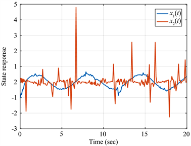
Figure 1. State variable response of open-loop system

图1. 开环系统状态变量响应

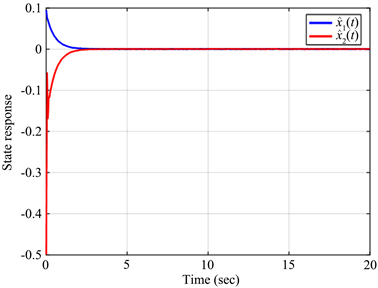
Figure 2. State variable response of closed-loop system

图2. 闭环系统状态变量响应

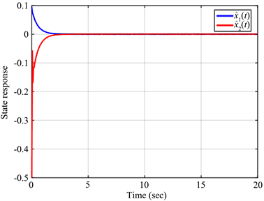
Figure 3. State estimation response of error system

图3. 误差系统状态估计响应

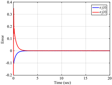
Figure 4. Response of error system state variables

图4. 误差系统状态变量响应

Figure 5. Sliding mode state response

图5. 滑模状态响应

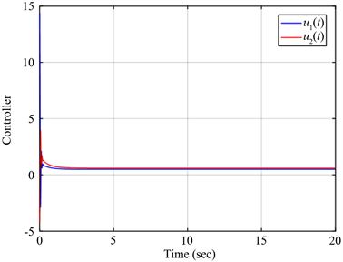
Figure 6. Control system state variable response

图6. 控制系统状态变量响应

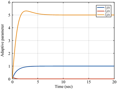
Figure 7. Adaptive parameter variable response

图7. 自适应参数变量响应

在初始条件 $x_0=\left[\begin{array}{cc}1& 0\end{array}\right]$ 和 ${\hat{x}}_0={\left[\begin{array}{cc}0.2& 0.3\end{array}\right]}^{\text{T}}$ 下的仿真结果如图1~图6所示，由图1~图2所示：闭环系统的状态响应要优于开环系统的；由图5所示：状态变量沿着控制轨迹到达滑模面的时间为2 s左右。综上所述，本文所提出的方法时有效且良好的。

本文方法仅对系统(1)有效，当系统(1)涉及到时间延迟、传感器故障、执行器故障等问题，结论不再适用。因此，系统(1)的容错控制和有限时间控制结合以上性能缺陷可以认为是今后的研究方向。

6. 结论

在本文的研究工作中，介绍了研究该系统的背景与意义，给出了系统模型及假设；针对该系统，通过设计了可行的滑模面函数，以此求得等效控制器，并得到了闭环系统。又设计一种新的自适应滑模控制率，用于保证滑模面的有限时间可达性。最后，利用LMI和李雅普诺夫函数理论，分别得到闭环系统带有 $H_{\infty }$ 扰动衰减水平的容许性的充分条件。

基金项目

国家自然科学基金项目(61074005)和辽宁省高等教育人才工程(LR2012005)。

NOTES

^*通讯作者。