任意凸四边形区域上二阶椭圆特征值问题基于高阶多项式逼近的一种数值方法

A Numerical Method Based on Higher Order Polynomial Approximation for Second Order Elliptic Eigenvalue Problems on Arbitrary Convex Quadrilateral Domain

摘要: 提出了任意凸四边形区域上二阶椭圆特征值问题基于高阶多项式逼近的一种有效的数值方法。首先，利用等参变换将任意凸四边形区域上的函数转化为变[-1,1]Χ[-1,1]上的函数，并建立原问题在等参变换下的弱形式及其逼近格式。其次，利用Legendre正交多项式的性质构造逼近空间中有效的一组基函数，将逼近格式转化为基于矩阵形式的线性特征系统，从而可以通过MATLAB软件编程求解出相应的特征值。最后，一些数值算例被呈现，数值结果进一步验证了我们算法的有效性和收敛性。

Abstract: An effective numerical method based on high-order polynomial approximation for second-order elliptic eigenvalue problems on arbitrary convex quadrilateral regions is proposed. Firstly, the function on any convex quadrilateral region is transformed into a function on variable by isoparametric transformation, and the weak form and approximation scheme of the original problem under isoparametric transformation are established. Secondly, a set of effective basis functions in the approximation space are constructed by using the properties of Legendre orthogonal polynomials, and the approximation format is transformed into a linear characteristic system based on matrix form, so that the corresponding eigenvalues can be solved by MATLAB software programming. Finally, some numerical examples are presented, and the numerical results further verify the effectiveness and convergence of our algorithm.

1. 引言

在很多工程和科学领域，特征值问题有着广泛的应用，如量子力学、流体力学和随机过程 [1] [2] [3] [4] [5] 等。关于特征值问题的数值计算，已经有各种各样的数值方法，主要包括三角域谱方法 [6] [7] [8] [9]、一些混合元法和杂交元法 [10] [11]、有限元方法 [12] [13] [14] [15] [16] 和有限差分法 [17]。随后，一些谱方法也相继被提出，例如文献 [18] 中李艳琴等人利用有效的谱Galerkin方法，解决了矩形区域上的四阶椭圆特征值问题；文献 [19] 中安静提出了基于Legendre-Galerkin逼近的一种有效的谱方法，研究了Steklov特征值问题。然而，根据我们了解，关于任意凸四边形区域上二阶椭圆特征值问题基于高阶多项式逼近的报道较少。从而，本文提出了任意凸四边形区域上二阶椭圆特征值问题基于高阶多项式逼近的一种有效的数值方法。首先，利用等参变换将任意凸四边形区域上的函数转化为变 $\left[-1,1\right]\times \left[-1,1\right]$ 上的函数，并建立原问题在等参变换下的弱形式及其逼近格式。其次，利用Legendre正交多项式的性质构造逼近空间中的一组基函数，将逼近格式转化为基于矩阵形式的线性特征系统，从而可以通过MATLAB软件编程求解出相应的特征值。最后，一些数值算例被呈现，数值结果进一步验证了我们算法的有效性和收敛性，进一步表明了我们的算法是合理的。

本文的其它内容如下：在第2节，我们建立了任意凸四边形区域上二阶椭圆特征值问题的弱形式及其逼近格式。在第3节，我们详细地描述了算法的有效实现。在第4节，我们给出了一些数值算例。在第5节，我们给出了一些结论性评注。

2. 弱形式和逼近格式

作为一个模型问题，我们考虑下面的二阶椭圆特征值问题：

$\{\begin{array}{l}-\Delta u+\alpha u=\lambda u,\left(x,y\right)\in \Omega \\ {u|}_{\partial \Omega }=0,\left(x,y\right)\in \partial \Omega \end{array}$ (1)

其中 $\alpha$ 为非负常数。

首先，设任意凸四边形区域 $\Omega$ 的顶点坐标分别为 $\left(x_1,y_1\right),\left(x_2,y_2\right),\left(x_3,y_3\right),\left(x_4,y_4\right)$，作 $\Omega$ 的一个双线性等参变换：

$\{\begin{array}{l}x\left(\zeta ,\eta \right)=x_1+\left(x_2-x_1\right)\zeta +\left(x_3-x_1\right)\eta +\left(x_4-x_3-x_2-x_1\right)\zeta \eta ,\\ y\left(\zeta ,\eta \right)=y_1+\left(y_2-y_1\right)\zeta +\left(y_3-y_1\right)\eta +\left(y_4-y_3-y_2-y_1\right)\zeta \eta ,\end{array}$ (2)

其中 $0\le \zeta ,\eta \le 1$。则(1)可化为如下的等价形式：

$\{\begin{array}{l}-\Delta \tilde{u}+\alpha \tilde{u}=\lambda \tilde{u},\left(\zeta ,\eta \right)\in D,\\ {\tilde{u}|}_{\partial D}=0,\end{array}$ (3)

其中 $\tilde{u}\left(\zeta ,\eta \right)=u\left(x,y\right),D=\left(0,1\right)\times \left(0,1\right)$。

为了保证是凸区域上的等参变换是一对一的，变换 $x=x\left(\zeta ,\eta \right),y=y\left(\zeta ,\eta \right)$ 的Jacobi行列式需要满足下列条件：

$J=\left|\begin{array}{cc}{x}_2-x_1+a\eta & x_3-x_1+a\zeta \\ y_2-y_1+b\eta & y_3-y_1+b\zeta \end{array}\right|>0,$ (4)

其中 $a=x_4-x_3-x_2+x_1,b=y_4-y_3-y_2+y_1$。

令 $H_0^1\left(D\right)$ 表示通常的Sobolev空间，则由格林公式可得(3)的弱形式为：求 $\left(\lambda ,\tilde{u}\right)\in ℝ\times H_0^1\left(D\right)$，使得：

$a\left(\tilde{u},v\right)=\lambda b\left(\tilde{u},v\right),\forall v\in H_0^1\left(D\right),$ (5)

其中： $a\left(\tilde{u},v\right)={\displaystyle {\int }_D\nabla \tilde{u}\nabla v}J\text{d}\zeta \text{d}\eta +\alpha {\displaystyle {\int }_D\tilde{u}vJ}\text{d}\zeta \text{d}\eta ,b\left(\tilde{u},v\right)={\displaystyle {\int }_D\tilde{u}vJ}\text{d}\zeta \text{d}\eta$。

将(5)进一步化为如下的等价形式：

$\begin{array}{l}{\displaystyle {\int }_D[\left(\frac{\partial \tilde{u}}{\partial \zeta }\frac{\partial \zeta }{\partial x}+\frac{\partial \tilde{u}}{\partial \eta }\frac{\partial \eta }{\partial x}\right)\left(\frac{\partial v}{\partial \zeta }\frac{\partial \zeta }{\partial x}+\frac{\partial v}{\partial \eta }\frac{\partial \eta }{\partial x}\right)}+\left(\frac{\partial \tilde{u}}{\partial \zeta }\frac{\partial \zeta }{\partial y}+\frac{\partial \tilde{u}}{\partial \eta }\frac{\partial \eta }{\partial y}\right)\\ \times \left(\frac{\partial v}{\partial \zeta }\frac{\partial \zeta }{\partial y}+\frac{\partial v}{\partial \eta }\frac{\partial \eta }{\partial y}\right)]\frac{1}{J}\text{d}\zeta \text{d}\eta +\alpha {\displaystyle {\int }_D\tilde{u}vJ\text{d}\zeta \text{d}\eta }=\lambda {\displaystyle {\int }_D\tilde{u}v}J\text{d}\zeta \text{d}\eta .\end{array}$ (6)

为了能够使用 $\left[-1,1\right]$ 上的正交多项式逼近，我们需要进一步引入坐标变换：

$\{\begin{array}{l}\zeta =\frac{1}{2}\left(t+1\right),t\in \left[-1,1\right],\\ \eta =\frac{1}{2}\left(\tau +1\right),\tau \in \left[-1,1\right].\end{array}$

令 $\hat{u}\left(t,\tau \right)=\tilde{u}\left(\zeta ,\eta \right),\hat{D}=\left(-1,1\right)\times \left(-1,1\right)$。由于

$\{\begin{array}{l}\frac{\partial \zeta }{\partial x}=\frac{\partial y}{\partial \eta }\frac{1}{J},\frac{\partial \eta }{\partial x}=-\frac{\partial y}{\partial \zeta }\frac{1}{J},\\ \frac{\partial \eta }{\partial y}=\frac{\partial x}{\partial \zeta }\frac{1}{J},\frac{\partial \zeta }{\partial y}=-\frac{\partial x}{\partial \eta }\frac{1}{J}.\end{array}$ (7)

从而(7)可化为如下的等价形式：

$\begin{array}{l}{\displaystyle {\int }_{\hat{D}}[{\hat{u}}_t{v}_t{\left(y_3-y_1+\frac{b\left(t+1\right)}{2}\right)}^2}-{\hat{u}}_t{v}_{\tau }\left(y_3-y_1+\frac{b\left(t+1\right)}{2}\right)\left(y_2-y_1+\frac{b\left(\tau +1\right)}{2}\right)\\ -{\hat{u}}_{\tau }{v}_t\left(y_3-y_1+\frac{b\left(t+1\right)}{2}\right)\left(y_2-y_1+\frac{b\left(\tau +1\right)}{2}\right)+{\hat{u}}_{\tau }{v}_{\tau }{\left(y_2-y_1+\frac{b\left(\tau +1\right)}{2}\right)}^2\\ +{\hat{u}}_{\tau }{v}_{\tau }{\left(x_2-x_1+\frac{a\left(\tau +1\right)}{2}\right)}^2-{\hat{u}}_{\tau }{v}_t\left(x_2-x_1+\frac{a\left(\tau +1\right)}{2}\right)\left(x_3-x_1+\frac{a\left(t+1\right)}{2}\right)\\ -{\hat{u}}_t{v}_{\tau }\left(x_3-x_1+\frac{a\left(t+1\right)}{2}\right)\left(x_2-x_1+\frac{a\left(\tau +1\right)}{2}\right)+{\hat{u}}_t{v}_t{\left(y_3-y_1+\frac{a\left(t+1\right)}{2}\right)}^2]\\ \times \frac{1}{J}\text{d}t\text{d}\tau +\frac{\alpha }{4}{\displaystyle {\int }_{\hat{D}}\hat{u}v}J\text{d}t\text{d}\tau =\frac{\lambda }{4}{\displaystyle {\int }_{\hat{D}}\hat{u}v}J\text{d}t\text{d}\tau .\end{array}$ (8)

定义逼近空间 $X_N=\left(P_N\times P_N\right)\cap H_0^1\left(\hat{D}\right)$，其中 $P_N$ 表示次数不超过N的多项式空间。则(8)相应的逼近格式为：找 $\left({\lambda }_N,{\hat{u}}_N\right)\in ℝ\times X_N$，使得：

$\begin{array}{l}{\displaystyle {\int }_{\hat{D}}[{\hat{u}}_{Nt}{v}_{Nt}{\left(y_3-y_1+\frac{b\left(t+1\right)}{2}\right)}^2}-{\hat{u}}_{Nt}{v}_{N\tau }\left(y_3-y_1+\frac{b\left(t+1\right)}{2}\right)\left(y_2-y_1+\frac{b\left(\tau +1\right)}{2}\right)\\ -{\hat{u}}_{N\tau }{v}_{Nt}\left(y_3-y_1+\frac{b\left(t+1\right)}{2}\right)\left(y_2-y_1+\frac{b\left(\tau +1\right)}{2}\right)+{\hat{u}}_{N\tau }{v}_{N\tau }{\left(y_2-y_1+\frac{b\left(\tau +1\right)}{2}\right)}^2\\ +{\hat{u}}_{N\tau }{v}_{N\tau }{\left(x_2-x_1+\frac{a\left(\tau +1\right)}{2}\right)}^2-{\hat{u}}_{N\tau }{v}_{Nt}\left(x_2-x_1+\frac{a\left(\tau +1\right)}{2}\right)\left(x_3-x_1+\frac{a\left(t+1\right)}{2}\right)\\ -{\hat{u}}_{Nt}{v}_{N\tau }\left(x_3-x_1+\frac{a\left(t+1\right)}{2}\right)\left(x_2-x_1+\frac{a\left(\tau +1\right)}{2}\right)+{\hat{u}}_{Nt}{v}_{Nt}{\left(y_3-y_1+\frac{a\left(t+1\right)}{2}\right)}^2]\\ \times \frac{1}{J}\text{d}t\text{d}\tau +\frac{\alpha }{4}{\displaystyle {\int }_{\hat{D}}{\hat{u}}_N{v}_N}J\text{d}t\text{d}\tau =\frac{\lambda }{4}{\displaystyle {\int }_{\hat{D}}{\hat{u}}_N{v}_N}J\text{d}t\text{d}\tau ,\forall v_N\in X_N.\end{array}$ (9)

3. 算法的有效实现

在这一节，我们将描述算法的实现过程。首先，我们构造逼近空间 $X_N$ 的一组基函数。令 ${\psi }_k\left(t\right)=L_k\left(t\right)-L_{k+2}\left(t\right)\left(k=0,1,2,\cdots ,N-2\right)$，其中 $L_k\left(t\right)$ 为k次Legendre多项式，则逼近空间 $X_N$ 可表示为：

$X_N=span\left\{{\psi }_i\left(t\right){\psi }_j\left(\tau \right):i,j=0,1,2,\cdots ,N-2\right\}.$ (10)

将 ${\hat{u}}_N$ 用基函数展开得：

${\hat{u}}_N={\displaystyle \underset{i,j=0}{\overset{N-2}{\sum }}{u}_{ij}{\psi }_i\left(t\right){\psi }_j\left(\tau \right)}$ (11)

其中 $u_{ij}$ 为展开系数。令

$U=\left(\begin{array}{cccc}{u}_{00}& u_{01}& \cdots & u_{0,N-2}\\ u_{10}& u_{11}& \cdots & u_{1,N-2}\\ ⋮& ⋮& \ddots & ⋮\\ u_{N-2,0}& u_{N-2,1}& \cdots & u_{N-2,N-2}\end{array}\right).$ (12)

将(11)代入(9)，在(9)中让 $v_N$ 取遍逼近空间 $X_N$ 中所有的基函数，通过一系列的推导和整理得：

$AU=\lambda {}_{N}BU.$ (13)

其中：

$\begin{array}{l}A=A_{sm}^1-A_{sm}^2-A_{sm}^3+A_{sm}^4+A_{sm}^5-A_{sm}^6-A_{sm}^7+A_{sm}^8+\alpha B_{sm},\\ B=B_{sm},A_{sm}^k={\left(s_{mi}^k{m}_{nj}^k\right)}_{m,i,n,j=0}^{N-2},k=1,2,\cdots ,8,B_{sm}={\left(s_{mi}{m}_{nj}\right)}_{m,i,n,j=0}^{N-2}.\end{array}$

$s_{mi}^1{m}_{nj}^1=4{\displaystyle {\int }_{-1}^1{\displaystyle {\int }_{-1}^1{{\psi }^{\prime }}_i}}\left(t\right){\psi }_j\left(\tau \right){{\psi }^{\prime }}_m\left(t\right){\psi }_n\left(\tau \right){\left[y_3-y_1+b\frac{t+1}{2}\right]}^2\frac{1}{J}\text{d}t\text{d}\tau ,$

$s_{mi}^2{m}_{nj}^2=4{\displaystyle {\int }_{-1}^1{\displaystyle {\int }_{-1}^1{{\psi }^{\prime }}_i}}\left(t\right){\psi }_j\left(\tau \right){\psi }_m\left(t\right){{\psi }^{\prime }}_n\left(\tau \right)\left[y_3-y_1+b\frac{t+1}{2}\right]\times \left[y_2-y_1+b\frac{\tau +1}{2}\right]\frac{1}{J}\text{d}t\text{d}\tau ,$

$s_{mi}^3{m}_{nj}^3=4{\displaystyle {\int }_{-1}^1{\displaystyle {\int }_{-1}^1{\psi }_i}}\left(t\right){{\psi }^{\prime }}_j\left(\tau \right){{\psi }^{\prime }}_m\left(t\right){\psi }_n\left(\tau \right)\left[y_2-y_1+b\frac{\tau +1}{2}\right]\times \left[y_3-y_1+b\frac{t+1}{2}\right]\frac{1}{J}\text{d}t\text{d}\tau ,$

$s_{mi}^4{m}_{nj}^4=4{\displaystyle {\int }_{-1}^1{\displaystyle {\int }_{-1}^1{\psi }_i}}\left(t\right){{\psi }^{\prime }}_j\left(\tau \right){\psi }_m\left(t\right){{\psi }^{\prime }}_n\left(\tau \right){\left[y_2-y_1+b\frac{\tau +1}{2}\right]}^2\frac{1}{J}\text{d}t\text{d}\tau ,$

$s_{mi}^5{m}_{nj}^5=4{\displaystyle {\int }_{-1}^1{\displaystyle {\int }_{-1}^1{\psi }_i}}\left(t\right){{\psi }^{\prime }}_j\left(\tau \right){\psi }_m\left(t\right){{\psi }^{\prime }}_n\left(\tau \right){\left[x_2-x_1+a\frac{\tau +1}{2}\right]}^2\frac{1}{J}\text{d}t\text{d}\tau ,$

$s_{mi}^6{m}_{nj}^6=4{\displaystyle {\int }_{-1}^1{\displaystyle {\int }_{-1}^1{\psi }_i}}\left(t\right){{\psi }^{\prime }}_j\left(\tau \right){{\psi }^{\prime }}_m\left(t\right){\psi }_n\left(\tau \right)\left[x_2-x_1+a\frac{\tau +1}{2}\right]\times \left[x_3-x_1+a\frac{t+1}{2}\right]\frac{1}{J}\text{d}t\text{d}\tau ,$

$s_{mi}^7{m}_{nj}^7=4{\displaystyle {\int }_{-1}^1{\displaystyle {\int }_{-1}^1{{\psi }^{\prime }}_i}}\left(t\right){\psi }_j\left(\tau \right){\psi }_m\left(t\right){{\psi }^{\prime }}_n\left(\tau \right)\left[x_3-x_1+a\frac{t+1}{2}\right]\times \left[x_2-x_1+a\frac{\tau +1}{2}\right]\frac{1}{J}\text{d}t\text{d}\tau ,$

$s_{mi}^8{m}_{nj}^8=4{\displaystyle {\int }_{-1}^1{\displaystyle {\int }_{-1}^1{{\psi }^{\prime }}_i}}\left(t\right){\psi }_j\left(\tau \right){{\psi }^{\prime }}_m\left(t\right){\psi }_n(\tau ){\left[x_3-x_1+a\frac{t+1}{2}\right]}^2\frac{1}{J}\text{d}t\text{d}\tau ,$，

$s_{mi}{m}_{nj}={\displaystyle {\int }_{-1}^1{\displaystyle {\int }_{-1}^1{\psi }_i}}\left(t\right){\psi }_j\left(\tau \right){\psi }_m\left(t\right){\psi }_n\left(\tau \right)J\text{d}t\text{d}\tau .$

4. 数值算例

为了表明算法的有效性和收敛性，一系列数值算例被呈现，我们将在MATLAB 2019a平台上进行编程测试。

例1我们取 $\alpha =0$， $\Omega =\left[0,1\right]\times \left[0,1\right]$ 时，该问题的精确特征值为 $\lambda =k^2{\pi }^2$，则前四个特征值分别为：

${\lambda }_{{}^1}=\text{19}\text{.739208802178716},{\lambda }_{{}^2}=\text{49}\text{.348022005446794},$

${\lambda }_{{}^3}=\text{49}\text{.348022005446794},{\lambda }_{{}^4}=\text{78}\text{.956835208714864}.$

我们在表1中列出了前四个特征值的数值结果(见表1)。

Table 1. Numerical results for different N first four eigenvalues

表1. 对于不同的N前4个特征值的数值结果

从表1可以观察到，当 $N\ge 25$ 时，前四个特征值达到了至少14位有效数字的精度。为了进一步表明算法的收敛性，对于不同的N，在图1中画出了逼近特征值与精确特征值之间的误差曲线，从而图1也观察到我们的算法是收敛性。

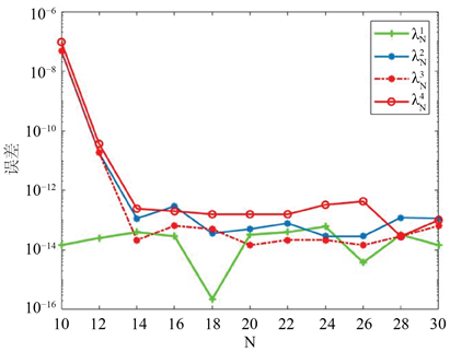
Figure 1. Error curve between approximate eigenvalue and exact eigenvalue

图1. 逼近特征值与精确特征值之间的误差曲线

例2我们考虑 $\Omega$ 为一般的凸四边形区的情况。取 $\alpha =0$，四个顶点坐标分别为： $A\left(x_1,y_1\right)=A\left(-2,-1\right)$， $B\left(x_2,y_2\right)=B\left(2,-3\right)$， $C\left(x_3,y_3\right)=C\left(-1,1.25\right)$， $D\left(x_4,y_4\right)=D\left(2,1\right)$，如图2所示。我们在表2中列出了前四个特征值的数值结果(见表2)。

从表2可以看出，当 $N\ge 30$ 时，前四个特征值达到了至少6位有效数字的精度。为了进一步表明算法的有效性，我们取 $N=60$ 时的数值解作为参考解，对于不同的N，在图3中画出了逼近特征值与参考解之间的误差曲线，从图3观察到我们算法也是收敛的。

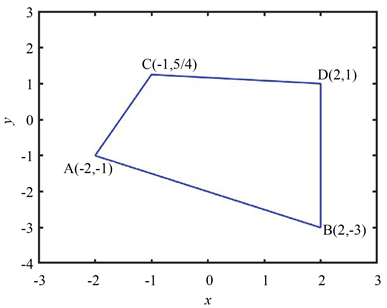
Figure 2. General convex quadrilateral region

图2. 一般的凸四边形区域

Table 2. Numerical results of the first four eigenvalues for different N

表2. 对于不同的N，前4个特征值的数值结果

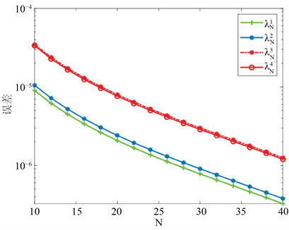
Figure 3. Error curve between approximate eigenvalue and reference solution

图3. 逼近特征值与参考解之间的误差曲线

5. 结论

针对二阶椭圆特征值问题，提出了任意凸四边形区域上二阶椭圆特征值问题基于高阶多项式逼近的一种有效的数值方法。通过等参变换和仿射变换将任意凸四边形区域变换到矩形区域 ${\left[-1,1\right]}^2$，再利用正交多项式逼近进行编程求解。从数值结果我们观察到，对于规则的矩形区域，数值特征值收敛很快，而且具有谱精度。对于不规则凸四边形区域，由于在尖角处解的正则性较低，所以收敛速度要慢一些，因此，本文提出的算法还可以利用谱元法进一步改进和优化，这是我们将来要思考和研究的工作。