基于无相位近场的非线性积分方程方法重构粗糙曲面

Reconstructions of a Rough Surface Based on a Nonlinear Integral Equation Method from Phaseless Near-Field Data

摘要: 本文研究第三类边界条件无穷粗糙曲面反散射问题。入射场uⁱ选取不同位置点源叠加的形式，点源打到散射曲面上产生散射场u^s，因此测量得到无相位近场|u|(|u|=|uⁱ+u^s|)，于是我们利用无相位近场的非线性积分方程方法重构无穷粗糙曲面的位置和形状。该算法的有效性通过数值算例实现。

Abstract: This paper studies the inverse scattering problem of infinite rough surfaces with boundary condition of the third kind. The incoming field uⁱ is taken as a sum of different position source points shooting at the scattering surface, which induces the scattered field u^s. Then we reconstruct infinite rough surfaces by a nonlinear integral equation method from the phaseless near field |u|(|u|=|uⁱ+u^s|). Numerical examples are presented to show the effectiveness of the inverse algorithm.

1. 绪论

在本篇文章中，我们研究无相位近场的第三类边界条件无穷粗糙曲面反散射问题。此类问题在诸如石油勘探、医学成像、信号处理、无损探测、工业控制等领域都有着广泛的应用前景和实际意义。

我们研究的第三类边界条件无穷粗糙曲面散射问题由两部分组成。第一部分是正散射问题，即已知入射场和散射曲面决定散射场。目前已有大量的研究工作比如积分方程方法 [1] - [7] 和变分法 [8] 说明了正散射问题的适定性，并且实现了正散射问题的数值计算，例如基于积分方程方法的Nystöm方法 [9] 和基于变分法的有限元方法 [10]。

第二部分则是反散射问题，即是通过测量远场或者近场来确定未知粗糙曲面的形状、位置以及物理属性的一类问题。反散射问题的数值算法主要有两大类，第一类为非迭代算法，例如线性采样方法 [11]、时域点源法 [12] 和时域探测法 [13]。第二类是迭代算法，例如非线性积分方程方法 [14] [15]、Kirsch-Kress方法 [16] [17]、牛顿类型的迭代算法 [7] [18] 和基于变换场展开的逆算法 [19] [20]，此类方法的优点在于如果选取适当的初始猜测值，往往能得到非常精确的重构效果。本篇文章所用的方法即迭代算法中的非线性积分方程方法。

上述所说的反散射问题数值算法是基于我们能够获得近场或者远场的强度和相位信息。在本篇文章中，我们是利用无相位近场重构第三类边界条件粗糙曲面的形状和位置，这是因为在实际应用问题中我们很难甚至测不到数据的相位信息。于是利用无相位的测量数据来重构散射体吸引了众多学者的关注，并取得了大量的研究进展 [21] - [39]。但是利用无相位测量数据重构散射体面临的挑战是只用一个平面波作为入射场所产生的无相位远场满足平移不变性 [26] [30]，即散射体任意平移前后所对应的无相位远场相同，这就导致利用无相位远场只能重构散射体的形状而无法重构其位置。在文献 [21] [22] [23] [24] [25] [27] [28] 中，我们得知利用无相位远场可以很好地重构散射体的形状。

目前，广泛应用于打破平移不变性的方法有两种，一种是在文献 [38] [39] 中，证明了由两个平面波叠加作为入射场产生的无相位远场不满足平移不变性，并利用此方法在无相位远场反散射问题取得了进一步突破，例如在文献 [34] 中证明了在单波数情形下由无穷多组两个平面波叠加作为入射场产生的无相位远场可以唯一确定散射体的形状和位置。另一种打破平移不变性的方法是在反散射问题模型中加入一个参考球组成一个整体由此唯一决定散射体 [29] [31] [32] [35] [36]。

虽然在文献 [33] [37] 中证明了以两个不同位置的点源入射所产生的无相位远场可以唯一确定散射体的位置，并且在文献 [36] 中表明点源叠加入射产生的无相位近场可以唯一决定局部扰动的粗糙曲面，但是我们没有获得多个点源叠加入射产生的无相位近场能否唯一决定全局扰动的粗糙曲面的理论证明。在本篇文章中，我们实现了在多波数情形下，利用多个点源叠加入射所产生的无相位近场重构无穷粗糙曲面的形状和位置的数值算法。通过文献 [6] 我们得知散射场由一个积分方程表示，于是由近场为入射场和散射场之和可知近场的表达形式，对其关于粗糙曲面和阻尼函数求Fréchet导数可获得关于粗糙曲面的近似Fréchet导数，由此我们提出了无相位近场的非线性积分方程方法。为了解决反散射问题的不适定性，我们利用多个波数，由此得到更精确的重构曲面，其迭代算法可以简述为给定在第一个波数下粗糙曲面和阻尼函数的初始猜测，通过无相位近场的非线性积分方程方法重构出第一个波数下的粗糙曲面，并作为第二个波数的初始猜测，由此进行下去直到迭代完所有波数以及满足停止准则。

这篇文章的第二部分构建了无相位近场的第三类边界条件无穷粗糙曲面散射问题的模型，并在第三部分提出无相位近场的非线性积分方程方法。第四部分则展示数值算例说明该算法的有效性。

2. 模型建立

我们将在这部分建立第三类边界条件无穷粗糙曲面反散射问题的数学模型，并给出散射场的积分表达。

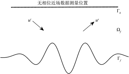
Figure 1. The geometry of the scattering problem

图1. 散射问题的几何表示

设函数空间 $B:=\left\{f\in C^{1,1}\left(ℝ\right)|f\left(s\right)\ge c_1,s\in ℝ,{\Vert f\Vert }_{C^{1,1}\left(ℝ\right)}\le c_2\right\}$，散射曲面 $\Gamma :=\left\{x=\left(x_1,x_2\right)\in {ℝ}^2:x_2=f\left(x_1\right),f\in B\right\}$，散射曲面上方的空间记为 $\Omega :=\left\{x=\left(x_1,x_2\right)\in {ℝ}^2:x_2>f\left(x_1\right),f\in B\right\}$，分别用 ${\Gamma }_f$ 和 ${\Omega }_f$ 表示 $\Gamma$ 和 $\Omega$ 依赖函数f， $\nu \left(x\right)$ 表示散射曲面 ${\Gamma }_f$ 的法向量，指向 ${\Omega }_f$ 的内部，函数空间 $R\left(\Omega \right):=\left\{w\left(x\right):w\left(x\right)\in C^2\left(\Omega \right)\cap C\left(\bar{\Omega }\right)\right\}$，在 $R\left(\Omega \right)$ 内定义法向导数为

$\frac{\partial w}{\partial \nu }\left(x\right):=\underset{h\to 0^{+}}{\lim }\nu \left(x\right)\cdot \nabla w\left(x+h\nu \left(x\right)\right)$， $x\in {\Gamma }_f$。

如图1所示，我们将第三类边界条件粗糙曲面散射问题表述为已知入射场 $u^i\in {\Omega }_f$ 和散射曲面 ${\Gamma }_f$，求解在 ${\Omega }_f$ 内满足Helmholtz方程的散射场 $u^s$ 且 $u^s\in R\left(\Omega \right)$，即

$\Delta u^s\left(x\right)+{\kappa }^2{u}^s\left(x\right)=0$， $x\in {\Omega }_f$， (2.1)

这里 $\kappa$ 表示波数。散射场 $u^s$ 在散射曲面 ${\Gamma }_f$ 满足第三类边界条件，即

${\partial }_{\nu }{u}^s+i\kappa \beta u^s=g$， (2.2)

其中 $g:=-\left({\partial }_{\nu }{u}^i+\text{i}\kappa \beta u^i\right)$，且 $g\in R\left(\Omega \right)$， $\beta$ 表示阻尼函数，是一个连续的复值函数。为了保证该散射问题的适定性，散射场 $u^s$ 满足向上传播条件：存在 $h>f_{+}:={\sup }_{x_1\in ℝ}f\left(x_1\right)$， $\psi \in L^{\infty }\left({\Gamma }_h\right)$，使得

$u^s\left(x\right)=2{\displaystyle {\int }_{{\Gamma }_h}{\partial }_{y_2}\Phi \left(x,y\right)\psi \left(y\right)\text{d}s\left(y\right)}$， $x\in U_h$， (2.3)

其中 $\Phi \left(x,y\right)=\frac{i}{4}{H}_0^{\left(1\right)}\left(\kappa \left|x-y\right|\right)$ 是Helmholtz方程的基本解， $H_0^{\left(1\right)}$ 表示第一类Hankel函数。此外，散射场 $u^s$ 需满足以下两个条件：

1) 存在 $a\in ℝ$，使得

$\underset{x\in {\Omega }_f}{\sup }{x}_2^a\left|u^s\left(x\right)\right|\le \infty$ ； (2.4)

2) 存在 $\theta \in \left(0,1\right)$， $C_{\theta }>0$，使得

$\left|\nabla u^s\left(x\right)\right|\le C_{\theta }{\left[x_2-f\left(x_1\right)\right]}^{\theta -1}$， $x\in {\Omega }_b$， (2.5)

这里 ${\Omega }_b:={\Omega }_f\backslash \overline{U_b}$， $b=f_{+}+1$。于是(2.1)~(2.5)表示散射场满足第三类边界条件粗糙曲面散射问题。在本篇文章中，入射场 $u^i$ 选用点源叠加的形式，即

$u^i\left(x\right)={\displaystyle \underset{j=1}{\overset{m}{\sum }}\Phi \left(x,z_j\right)}={\displaystyle \underset{j=1}{\overset{m}{\sum }}\frac{\text{i}}{4}{H}_0^{\left(1\right)}\left(\kappa \left|x-z_j\right|\right)}$， $z_j\in {\Omega }_f$。 (2.6)

在介绍接下来的结论之前，我们先设 $V\subset {ℝ}^n$， $n=1,2$，M为常数， $BC\left(V\right):=\left\{w\left(x\right):\left|w\left(x\right)\right|\le M,w\left(x\right)\in C\left(V\right)\right\}$ ； $d_1,d_2$ 为大于0的常数； $\omega :\left[0,\infty \right)\to \left[0,\infty \right)$， ${\lim }_{s\to 0}\omega \left(s\right)=0$ ； $E:=\left\{\tilde{\beta }\in BC\left(ℝ\right):Re\left(\tilde{\beta }\left(s\right)\right)\ge d,s\in ℝ,{\Vert \tilde{\beta }\Vert }_{\infty }\le d_2,\left|\tilde{\beta }\left(s\right)-\tilde{\beta }\left(t\right)\right|\le \omega \left(\left|s-t\right|\right),s,t\in ℝ\right\}$ ； $G_i\left(x,y\right)$ 表示在上半平面 $U_0:=\left\{x=\left(x_1,x_2\right)\in {ℝ}^2:x_2>0\right\}$ 满足算子 $\Delta +{\kappa }^2$ 的阻尼格林函数。

定理2.1设 $f\in B$， $\tilde{\beta }\left(s\right):=\beta \left(s,f\left(s\right)\right)\in E$， $g\in BC\left({\Gamma }_f\right)$ ：散射问题(2.1)-(2.5)存在唯一解 $u^s\left(x\right)$，其表达形式为

$u^s\left(x\right)={\displaystyle {\int }_{{\Gamma }_f}\left[{\partial }_{\nu \left(y\right)}{G}_i\left(x,y\right)+\text{i}\kappa \beta \left(y\right)G_i\left(x,y\right)\right]u^s\left(y\right)\text{d}s\left(y\right)}-{\displaystyle {\int }_{{\Gamma }_f}{G}_i\left(x,y\right)g\left(y\right)\text{d}s\left(y\right)}$， $x\in {\Omega }_f$

且

$u^s\left(x\right)-2{\displaystyle {\int }_{{\Gamma }_f}\left[{\partial }_{\nu \left(y\right)}{G}_i\left(x,y\right)+\text{i}\kappa \beta \left(y\right)G_i\left(x,y\right)\right]u^s\left(y\right)\text{d}s\left(y\right)}=-2{\displaystyle {\int }_{{\Gamma }_f}{G}_i\left(x,y\right)g\left(y\right)\text{d}s\left(y\right)}$， $x\in {\Gamma }_f$

存在唯一解 ${u^s\left(x\right)|}_{{\Gamma }_f}$。

为了方便书写，我们引进积分算子的形式，记

$F_i{u}^s\left(x\right)={\displaystyle {\int }_{{\Gamma }_f}\left[{\partial }_{\nu \left(y\right)}{G}_i\left(x,y\right)+\text{i}\kappa \beta \left(y\right)G_i\left(x,y\right)\right]u^s\left(y\right)\text{d}s\left(y\right)}-{\displaystyle {\int }_{{\Gamma }_f}{G}_i\left(x,y\right)g\left(y\right)\text{d}s\left(y\right)}$，

则 $u^s\left(x\right)=F_i{u}^s\left(x\right)$， $x\in {\Omega }_f$。

3. 无相位近场的非线性积分方程方法

在这部分我们将通过无相位近场 $\left|u_{{\kappa }_j}\right|$ ( $j=1,2,\cdots ,n$ 且 ${\kappa }_1<{\kappa }_2<\cdots <{\kappa }_n$ )的非线性积分方程方法重构粗糙曲面的形状和位置。测量无相位近场的位置为 ${\Gamma }_b:=\left\{x=\left(x_1,x_2\right)\in {ℝ}^2:x_2=b>f_{+}\right\}$。

由定理2.1，我们定义密度函数 $\varphi \left(x\right):={u^s\left(x\right)|}_{{\Gamma }_f}$，则

$\varphi \left(x\right)-2{\displaystyle {\int }_{{\Gamma }_f}\left[{\partial }_{\nu \left(y\right)}{G}_i\left(x,y\right)+\text{i}\kappa \beta \left(y\right)G_i\left(x,y\right)\right]\varphi \left(y\right)\text{d}s\left(y\right)}=-2{\displaystyle {\int }_{{\Gamma }_f}{G}_i\left(x,y\right)g\left(y\right)\text{d}s\left(y\right)}$， (3.1)

利用Nystöm方法求解得到密度函数 $\varphi$，详细步骤参考 [15]。由(3.1)得到已知的密度函数 $\varphi$，则无相位近场

$\left|u\left(x\right)\right|=\left|u^i\left(x\right)+u^s\left(x\right)\right|=\left|u^i\left(x\right)+F_i\varphi \left(x\right)\right|$， $x\in {\Gamma }_b$。 (3.2)

综上，我们得出求解无相位近场的反散射问题等价于求解(3.1)和(3.2)。由于阻尼格林函数 $G_i\left(x,y\right)$ 计算极其复杂，所以我们选用Dirichlet格林函数 $G\left(x,y\right)=\Phi \left(x,y\right)-\Phi \left(x,y^{\prime }\right)$ 代替阻尼格林函数 $G_i\left(x,y\right)$，其中 $y=\left(y_1,y_2\right)$， $y=\left(y_1,-y_2\right)$，其可行性参考 [14]。于是(3.1)和(3.2)化为

$\varphi \left(x\right)-2{\displaystyle {\int }_{{}_{{\Gamma }_f}}\left[{\partial }_{\nu \left(y\right)}G\left(x,y\right)+\text{i}\kappa \beta \left(y\right)G\left(x,y\right)\right]\varphi \left(y\right)\text{d}s\left(y\right)}=-2{\displaystyle {\int }_{{\Gamma }_f}G\left(x,y\right)g\left(y\right)\text{d}s\left(y\right)}$， $x\in {\Gamma }_f$， (3.3)

我们记

$\begin{array}{c}F\varphi \left(x\right):={\displaystyle {\int }_{{}_{{\Gamma }_f}}\left[{\partial }_{\nu \left(y\right)}G\left(x,y\right)+\text{i}\kappa \beta \left(y\right)G\left(x,y\right)\right]\varphi \left(y\right)\text{d}s\left(y\right)}-{\displaystyle {\int }_{{\Gamma }_f}G\left(x,y\right)g\left(y\right)\text{d}s\left(y\right)}\\ =-\frac{\kappa \text{i}}{4}{\displaystyle {\int }_{ℝ}\frac{H_1^{\left(1\right)}\left(\kappa \left|x-y\right|\right)}{\left|x-y\right|}}\left[\left(x_1-y_1\right)f^{\prime }\left(y_1\right)+f\left(y_1\right)-x_2\right]\varphi \left(y_1\right)\text{d}{y}_1\\ +\frac{\kappa \text{i}}{4}{\displaystyle {\int }_{ℝ}\frac{H_1^{\left(1\right)}\left(\kappa \left|x-y^{\prime }\right|\right)}{\left|x-y^{\prime }\right|}}\left[\left(x_1-y_1\right)f^{\prime }\left(y_1\right)+f\left(y_1\right)+x_2\right]\varphi \left(y_1\right)\text{d}{y}_1\\ -\frac{\kappa }{4}{\displaystyle {\int }_{ℝ}\left[H_0^{\left(1\right)}\left(\kappa \left|x-y\right|\right)-H_0^{\left(1\right)}\left(\kappa \left|x-y^{\prime }\right|\right)\right]}\sqrt{1+{\left[f^{\prime }\left(y_1\right)\right]}^2}\beta \left(y_1\right)\varphi \left(y_1\right)\text{d}{y}_1\\ -\frac{\text{i}}{4}{\displaystyle {\int }_{ℝ}\left[H_0^{\left(1\right)}\left(\kappa \left|x-y\right|\right)-H_0^{\left(1\right)}\left(\kappa \left|x-y^{\prime }\right|\right)\right]}\sqrt{1+{\left[f^{\prime }\left(y_1\right)\right]}^2}g\left(y_1\right)\text{d}{y}_1\end{array}$

则

$\left|u\left(x\right)\right|=\left|A\varphi \right|=\left|u^i\left(x\right)+F\varphi \left(x\right)\right|$， $x\in {\Gamma }_b$， (3.4)

其中

$A\varphi :=u^i\left(x\right)+F\varphi \left(x\right)$， (3.5)

对(3.4)两边同时取平方，则有

$\left(A\varphi \overline{A\varphi }\right)\left(x\right)=\left(u\bar{u}\right)\left(x\right)$， $x\in {\Gamma }_b$。 (3.6)

由于(3.6)关于f和 $\beta$ 都是非线性的，求解f和 $\beta$ 我们需要将其线性化，即对(3.6)关于f， $\beta$ 分别在 $f^{\delta }$， ${\beta }^{\delta }$ 方向求Fréchet导数，于是我们有

${\left(A\varphi \overline{A\varphi }\right)}^{\prime }{f}^{\delta }\left(x\right)+{\left(A\varphi \overline{A\varphi }\right)}^{\prime }{\beta }^{\delta }\left(x\right)=u\left(x\right)\overline{u\left(x\right)}-A\varphi \left(x\right)\overline{A\varphi }\left(x\right)$， $x\in {\Gamma }_b$。 (3.7)

由文献 [31] [40] 关于Fréchet导数的计算，我们得出对积分算子求Fréchet导数只需对积分算子的积分核求Fréchet导数，于是有

${\left(A\varphi \overline{A\varphi }\right)}^{\prime }{f}^{\delta }\left(x\right)=2Re\left\{\overline{u^i\left(x\right)}\frac{\partial F\varphi }{\partial f}{f}^{\delta }\left(x\right)\right\}+2Re\left\{\overline{F\varphi \left(x\right)}\frac{\partial F\varphi }{\partial f}{f}^{\delta }\left(x\right)\right\}$

和

${\left(A\varphi \overline{A\varphi }\right)}^{\prime }{\beta }^{\delta }\left(x\right)=2Re\left\{\overline{u^i\left(x\right)}\frac{\partial F\varphi }{\partial \beta }{\beta }^{\delta }\left(x\right)\right\}+2Re\left\{\overline{F\varphi \left(x\right)}\frac{\partial F\varphi }{\partial \beta }{\beta }^{\delta }\left(x\right)\right\}$，

其中

$\begin{array}{c}\frac{\partial F\varphi }{\partial f}{f}^{\delta }\left(x\right)=\frac{\kappa {\text{i}}^2}{4}{\displaystyle {\int }_{ℝ}\frac{H_2^{\left(1\right)}\left(\kappa \left|x-y\right|\right)}{{\left|x-y\right|}^2}}\left[\left(x_1-y_1\right)f^{\prime }\left(y_1\right)+f\left(y_1\right)-x_2\right]\left[f\left(y_1\right)-x_2\right]f^{\delta }\left(y_1\right)\varphi \left(y_1\right)\text{d}{y}_1\\ -\frac{{\kappa }^2\text{i}}{4}{\displaystyle {\int }_{ℝ}\frac{H_2^{\left(1\right)}\left(\kappa \left|x-y^{\prime }\right|\right)}{{\left|x-y^{\prime }\right|}^2}}\left[\left(x_1-y_1\right)f^{\prime }\left(y_1\right)+f\left(y_1\right)+x_2\right]\left[f\left(y_1\right)+x_2\right]f^{\delta }\left(y_1\right)\varphi \left(y_1\right)\text{d}{y}_1\\ +\frac{\kappa \text{i}}{4}{\displaystyle {\int }_{ℝ}\left[-\frac{H_1^{\left(1\right)}\left(\kappa \left|x-y\right|\right)}{\left|x-y\right|}+\frac{H_1^{\left(1\right)}\left(\kappa \left|x-y^{\prime }\right|\right)}{\left|x-y^{\prime }\right|}\right]}\left[\left(x_1-y_1\right)f^{\delta }{\left(y_1\right)}^{\prime }+f^{\delta }\left(y_1\right)\right]\varphi \left(y_1\right)\text{d}{y}_1\\ +\frac{{\kappa }^2}{4}{\displaystyle {\int }_{ℝ}\frac{H_1^{\left(1\right)}\left(\kappa \left|x-y\right|\right)}{\left|x-y\right|}}\left[f\left(y_1\right)-x_2\right]\sqrt{1+{\left[f^{\prime }\left(y_1\right)\right]}^2}\beta \left(y_1\right)f^{\delta }\left(y_1\right)\varphi \left(y_1\right)\text{d}{y}_1\\ -\frac{{\kappa }^2}{4}{\displaystyle {\int }_{ℝ}\frac{H_1^{\left(1\right)}\left(\kappa \left|x-y^{\prime }\right|\right)}{\left|x-y^{\prime }\right|}}\left[f\left(y_1\right)+x_2\right]\sqrt{1+{\left[f^{\prime }\left(y_1\right)\right]}^2}\beta \left(y_1\right)f^{\delta }\left(y_1\right)\varphi \left(y_1\right)\text{d}{y}_1\end{array}$

$\begin{array}{l}-\frac{\kappa }{4}{\displaystyle {\int }_{ℝ}\left[H_0^{\left(1\right)}\left(\kappa \left|x-y\right|\right)-H_0^{\left(1\right)}\left(\kappa \left|x-y^{\prime }\right|\right)\right]}\frac{f^{\prime }\left(y_1\right)}{\sqrt{1+{\left[f^{\prime }\left(y_1\right)\right]}^2}}\beta \left(y_1\right)f^{\delta }{\left(y_1\right)}^{\prime }\varphi \left(y_1\right)\text{d}{y}_1\\ +\frac{\kappa \text{i}}{4}{\displaystyle {\int }_{ℝ}\frac{H_1^{\left(1\right)}\left(\kappa \left|x-y\right|\right)}{\left|x-y\right|}}\left[f\left(y_1\right)-x_2\right]\sqrt{1+{\left[f^{\prime }\left(y_1\right)\right]}^2}{f}^{\delta }\left(y_1\right)g\left(y_1\right)\text{d}{y}_1\\ -\frac{\kappa \text{i}}{4}{\displaystyle {\int }_{ℝ}\frac{H_1^{\left(1\right)}\left(\kappa \left|x-y^{\prime }\right|\right)}{\left|x-y^{\prime }\right|}}\left[f\left(y_1\right)+x_2\right]\sqrt{1+{\left[f^{\prime }\left(y_1\right)\right]}^2}{f}^{\delta }\left(y_1\right)g\left(y_1\right)\text{d}{y}_1\\ -\frac{\text{i}}{4}{\displaystyle {\int }_{ℝ}\left[H_0^{\left(1\right)}\left(\kappa \left|x-y\right|\right)-H_0^{\left(1\right)}\left(\kappa \left|x-y^{\prime }\right|\right)\right]}\frac{f^{\prime }\left(y_1\right)}{\sqrt{1+{\left[f^{\prime }\left(y_1\right)\right]}^2}}{f}^{\delta }{\left(y_1\right)}^{\prime }g\left(y_1\right)\text{d}{y}_1\end{array}$

类似的，

$\frac{\partial F\varphi }{\partial \beta }{\beta }^{\delta }\left(x\right)=-\frac{\kappa }{4}{\displaystyle {\int }_{ℝ}\left[H_0^{\left(1\right)}\left(\kappa \left|x-y\right|\right)-H_0^{\left(1\right)}\left(\kappa \left|x-y^{\prime }\right|\right)\right]}\sqrt{1+{\left[f^{\prime }\left(y_1\right)\right]}^2}{\beta }^{\delta }\left(y_1\right)\left[\varphi \left(y_1\right)+u^i\left(y_1\right)\right]\text{d}{y}_1$。

在这篇文章中，表示散射曲面 ${\Gamma }_f$ 的函数f，阻尼函数 $\beta$ 以及f的更新数据 $f^{\delta }$， $\beta$ 的更新数据 ${\beta }^{\delta }$ 由三次样条函数的线性组合表出。设 $N_1,N_2\in \mathbb{N}$， $q_1,q_2>0$，

$f\left(x\right)={\displaystyle \underset{j=1}{\overset{2N_1+2}{\sum }}{a}_j}{h}_j\left(x\right),\beta \left(x\right)=Re\beta \left(x\right)+\text{i}Im\beta \left(x\right)={\displaystyle \underset{j=1}{\overset{2N_2+2}{\sum }}{b}_j}{g}_j\left(x\right)+\text{i}{\displaystyle \underset{j=1}{\overset{2N_2+2}{\sum }}{c}_j}{g}_j\left(x\right)$， (3.8)

$f^{\delta }\left(x\right)={\displaystyle \underset{j=1}{\overset{2N_1+2}{\sum }}{a}_j^{\delta }}{h}_j\left(x\right),{\beta }^{\delta }\left(x\right)=Re{\beta }^{\delta }\left(x\right)+\text{i}Im{\beta }^{\delta }\left(x\right)={\displaystyle \underset{j=1}{\overset{2N_2+2}{\sum }}{b}_j^{\delta }}{g}_j\left(x\right)+\text{i}{\displaystyle \underset{j=1}{\overset{2N_2+2}{\sum }}{c}_j^{\delta }}{g}_j\left(x\right)$， (3.9)

其中

$h_j\left(x\right)=\{\begin{array}{ll}1,\hfill & j=1,\hfill \\ {\Omega }_3\left(\frac{x-w_j}{q}\right),\hfill & j\ne 1,\hfill \end{array}$

$g_j\left(x\right)=\{\begin{array}{ll}1,\hfill & j=1,\hfill \\ {\Omega }_3\left(\frac{x-v_j}{q}\right),\hfill & j\ne 1,\hfill \end{array}$

这里 $w_j\left(j=1,2,\cdots ,2N_1+1\right)$， $v_j\left(j=1,2,\cdots ,2N_2+1\right)$ 为均匀分布在x轴上−d到d的点， ${\Omega }_3\left(x\right)$ 为三次样条函数，即

${\Omega }_3\left(x\right)=\{\begin{array}{ll}\frac{1}{2}{\left|x\right|}^3-x^2+\frac{2}{3},\hfill & \left|x\right|\le 1,\hfill \\ -\frac{1}{6}{\left|x\right|}^3+x^2-2\left|x\right|+\frac{3}{4},\hfill & 1<\left|x\right|<2,\hfill \\ 0,\hfill & \left|x\right|\ge 2.\hfill \end{array}$

为了方便起见，我们定义列向量

$a={\left(a_1,\cdots ,a_{2N_1+2}\right)}^{\top },b={\left(b_1,\cdots ,b_{2N_2+2}\right)}^{\top },c={\left(c_1,\cdots ,c_{2N_2+2}\right)}^{\top }$，

$a^{\delta }={\left(a_1^{\delta },\cdots ,a_{2N_1+2}^{\delta }\right)}^{\top },b^{\delta }={\left(b_1^{\delta },\cdots ,b_{2N_2+2}^{\delta }\right)}^{\top },c^{\delta }={\left(c_1^{\delta },\cdots ,c_{2N_2+2}^{\delta }\right)}^{\top }$

和矩阵 $X=\left(a;b;c\right)$， $X^{\delta }=\left(a^{\delta };b^{\delta };c^{\delta }\right)$。

我们用 $x_i$ 表示在 ${\Gamma }_b$ 上 $Nb\in \mathbb{N}$ 个测量点，将 $x_i$ 和(3.8)，(3.9)式代入(3.7)式得到

$J{X}^{\delta }=r$， (3.10)

其中r是一个列向量，其元素为

$r_i=u\bar{u}\left(x_i\right)-{\left(A\left[f,\beta ,\varphi \right]\overline{A\left[f,\beta ,\varphi \right]}\right)}^{\prime }\left(x_i\right)$。

设矩阵

$J^f:=\left(J_{ij}^f\right)=\left({\left(A\left[f,\beta ,\varphi \right]\overline{A\left[f,\beta ,\varphi \right]}\right)}^{\prime }{h}_j\left(x_i\right)\right),i=1,2,\cdots ,Nb,j=1,2,\cdots ,2N_1+2$，

$J^{\beta }:=\left(J_{ij}^{\beta }\right)=\left({\left(A\left[f,\beta ,\varphi \right]\overline{A\left[f,\beta ,\varphi \right]}\right)}^{\prime }{g}_j\left(x_i\right)\right),i=1,2,\cdots ,Nb,j=1,2,\cdots ,2N_2+2$，

于是有 $J=\left[J^f;J^{\beta };i{J}^{\beta }\right]$。由于(3.5)式的积分核是光滑的，所以(3.5)式严重不适定，则(3.7)式和(3.10)式也具有同样的性质，所以我们需对(3.10)式进行Tikhonov正则化，得到正则化方程

$\left(J^{*}J+\alpha I\right)X^{\delta }=J^{*}r$， (3.11)

$J^{*}$ 为J的伴随矩阵， $\alpha$ 表示正则化参数。

接下来，我们说明无相位近场的非线性积分方程方法重构无穷粗糙曲面的迭代算法。为了使算法简洁明了，首先给出单波数情形无相位近场的非线性积分方程方法。

迭代算法1给定 ${\Gamma }_b$ 上测量得到关于粗糙曲面的无相位近场 $\left|u_{\kappa }\right|$ 以及截断误差 ${ϵ}_{\kappa }$ ：

1) 选定关于粗糙曲面的初始猜测 $f_{0,\kappa }$ 和阻尼函数的初始猜测 ${\beta }_{0,\kappa }$ ；

2) 已知 $f_{m,\kappa }$， ${\beta }_{m,\kappa }$， $m\ge 0$，在(3.3)式中运用Nystöm方法求解 ${\varphi }_{m,\kappa }$ ；

3) 通过以上两步，我们已经知道 $\left(f_{m,\kappa },{\beta }_{m,\kappa },{\varphi }_{m,\kappa }\right)$， $m\ge 0$，于是求得(3.11)的更新数据 $f_{\kappa }^{\delta }$ 和 ${\beta }_{\kappa }^{\delta }$，则 $f_{m+1,\kappa }=f_{m,\kappa }+f_{\kappa }^{\delta }$， ${\beta }_{m+1,\kappa }={\beta }_{m,\kappa }+{\beta }_{\kappa }^{\delta }$ ；

4) 重复2) 3) 步直到 $ϵ\left(\kappa ,f_{\kappa }\right):=\frac{{\Vert \left|u_{m+1,\kappa }\right|-\left|u_{\kappa }\right|\Vert }_2}{{\Vert \left|u_{\kappa }\right|\Vert }_2}\le {ϵ}_{\kappa }$，迭代停止。这里 $\left|u_{m+1,\kappa }\right|$ 和 $\left|u_{\kappa }\right|$ 分别表示近似粗糙曲面 $f_{m+1,\kappa }$ 和精确曲面f的无相位近场。

基于算法1，我们现在给出多波数情形无相位近场的非线性积分方程方法的迭代算法。

迭代算法2对于波数 ${\kappa }_1<{\kappa }_2<\cdots <{\kappa }_n$，给定在每个波数下测量得到关于粗糙曲面的无相位近场数据 $\left|u_{{\kappa }_l}\right|$， $l=1,2,\cdots ,n$，初始值 $f_0$，初始截断误差 ${ϵ}_0$ 以及下降率 $\rho \in \left(0,1\right)$ ：

1) 设 $\kappa ={\kappa }_l$，当 $l=1$ 时，令 $f_{0,{\kappa }_1}=f_0$， ${\beta }_{0,{\kappa }_1}={\beta }_0$， ${ϵ}_{{\kappa }_l}={ϵ}_0$，否则 $f_{0,{\kappa }_{l+1}}=f_{{\kappa }_l}$， ${\beta }_{0,{\kappa }_{l+1}}={\beta }_{{\kappa }_l}$， ${ϵ}_{{\kappa }_{l+1}}=\rho ϵ\left({\kappa }_l,f_{{\kappa }_l}\right)$，且 $f_{{\kappa }_l}$， ${\beta }_{{\kappa }_l}$ 和 $ϵ\left({\kappa }_l,f_{{\kappa }_l}\right)$ 已经通过算法1得出；

2) 令 $l=l+1$，若 $l\le n$ 重复第(1)步，否则迭代停止。

4. 数值算例

在这部分，我们将展示数值算例来说明第3部分算法1和算法2的有效性。在以下算例中，我们设置共同参数如下：

· 入射场 $u^i$ 为241个点源之和，点源所在位置为 $z_j=\left(-60+0.5j,2\right)$， $j=0,1,\cdots ,240$。求解(3.3)式密度函数 $\varphi$ 时，设置粗糙曲面的截断间隔为 $\left[-8\pi ,8\pi \right]$，步长 $h=\frac{\pi }{N}$，其中 $N=5\kappa$，波数 $\kappa =1,2,\cdots ,10$，在每个波长 $\lambda =\frac{2\pi }{\kappa }$ 放入10个等距节点。测量数据的高度为 $x_2=b=1.5$，取值范围从 $-8\pi$ 到 $8\pi$，步长 $hb=0.05\pi$。

· 在计算(3.8)和(3.9)式时，设置 $N_1=N_2=160$， $d=40$， $w_j=v_j=-40+0.5j$， $j=0,1,\cdots ,160$。(3.11)式中，多次数值实验表明取正则化参数 ${\alpha }_{m,\kappa }={\Vert \left|u_{m,\kappa }\right|-\left|u_{\kappa }\right|\Vert }_2^{\frac{1}{4}}$ 效果最好。为了说明算法的稳定性，我们在测量数据中加入噪音 $\epsilon \left(\epsilon =0\%,2\%,5\%\right)$，所以加入噪音的测量数据为

$\left|u_{\epsilon ,\kappa }\right|=\left|u_{\kappa }\right|+\epsilon \frac{{\Vert \left|u_{\kappa }\right|\Vert }_2}{{\Vert \mu \Vert }_2}\mu$，

其中 $\mu ={\mu }_1+i{\mu }_2$， ${\mu }_1$， ${\mu }_2$ 服从正态分布。在算法2中，设置下降率 $\rho =0.5$。

· 在图2，图3中，黑色虚线，红色虚线以及蓝色曲线分别表示粗糙曲面 ${\Gamma }_f$ 的初始猜测，重构曲面以及精确值。第一、二、三排图片分别表示没有加噪音，噪音为2%和5%的重构算例。

算例1我们首先重构一个只有局部扰动的粗糙曲面，其函数表达为

$f\left(x\right)=0.5+0.3\exp \left(-3{\left(x+5\right)}^2\right)+0.1\exp \left(-0.2{\left(x+4\right)}^2\right)+0.5\exp \left(-2{\left(x-4\right)}^2\right)$。 (4.1)

阻尼函数表达如下

$Re=0.5+0.3\exp \left(-3{\left(x+5\right)}^2\right)+0.1\exp \left(-0.02{\left(x+4\right)}^2\right)-0.5\exp \left(-{\left(x+4\right)}^2\right)$，

$Im=0.5+0.3\exp \left(-3{\left(x+5\right)}^2\right)-0.1\exp \left(-0.02{\left(x+4\right)}^2\right)+0.5\exp \left(-0.04{\left(x+4\right)}^2\right)$，

则 $\beta =Re+\text{i}Im$。

重构(4.1)式时，散射曲面和阻尼函数的初始猜测分别为 $f_0=0.5$ 和 ${\beta }_0=0$，测量数据没有加噪音和加入2%的噪音时，初始截断误差 ${ϵ}_0=0.007$，加入5%的噪音时， ${ϵ}_0=0.02$。

算例2这个算例我们重构一个无穷全局扰动的粗糙曲面，其函数表达为

$\begin{array}{c}f\left(x\right)=0.5+0.3\cos \left(0.5\pi x\right)\exp \left(-0.05x^2\right)+0.2\sin \left(0.5\pi x\right)\exp \left(-0.05{\left(x-3\right)}^2\right)\\ -0.2\sin \left(\pi x\right)\exp \left(-0.05{\left(x+5\right)}^2\right)。\end{array}$ (4.2)

阻尼函数表达如下

$Re=Im=\sin x$，

则 $\beta =Re+\text{i}Im$。

算例2中散射曲面和阻尼函数的初始猜测分别为 $f_0=0.8$， ${\beta }_0=0$。测量数据没有加噪音和加入2%的噪音时，初始截断误差 ${ϵ}_0=0.02$，加入5%的噪音时， ${ϵ}_0=0.06$。

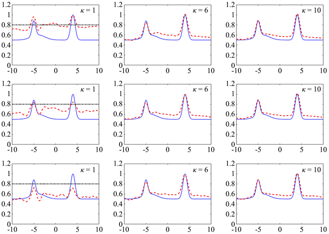
Figure 2. Reconstruction of (4.1) from data with no noise, 2% noise, 5% noise

图2. 局部粗糙曲面(4.1)的重构，噪音为0%，2%，5%

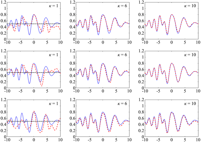
Figure 3. Reconstruction of (4.2) from data with no noise, 2% noise, 5% noise

图3. 局部粗糙曲面(4.2)的重构，噪音0%，2%，5%

5. 结论

本文实现了多频点源叠加入射产生的无相位近场的非线性积分方程方法重构第三类边界条件无穷粗糙曲面的数值算法，并且表明该散射问题等价于求解两个联立的积分方程组。数值实例表明点源叠加入射产生的无相位近场不满足平移不变性，在接下来的工作中，我们将致力于研究点源叠加入射产生的无相位近场不满足平移不变性的理论证明。

致谢

本篇文章是在导师李建樑副教授的悉心指导下完成，在此真诚地感谢李老师的帮助。在论文的撰写与修改过程中，李老师严谨细致，诲人不倦，我将受益终身。

NOTES

Email: [e-mail]