向列相液晶流的一种二阶全离散格式

A Second-Order Fully Discrete Scheme for Nematic Liquid Crystal Flow

摘要: 在本文中，我们对向列相液晶流的Ginzburg-Landau模型提出了一种二阶、线性、耦合的格式，证明了该格式在离散条件下的能量稳定性，最后，通过数值模拟展示了四奇异点和旋转流的湮没过程，并且验证了格式的数值精度。结果表明：该格式具有能量稳定性，且具有比较好的数值精度。

Abstract: In this paper, we mainly propose and analyze a second-order, linear, coupled scheme for the Ginzburg-Landau model of the nematic liquid crystal flow, and prove its energy stability under discrete condition. Finally, we demonstrate the annihilation process of four singularities and rotating flows through numerical simulations, and verify the numerical accuracy of the scheme. The results show that the scheme has energy stability and good numerical accuracy.

1. 引言

液晶被称为物质的第四种状态，不同于液体、固体、气体，它是一种兼有固体和液体性质的中间态，称为中间相。液晶显示(LCD)材料常用于数字手表和计算器显示板的制作，它们有明显的优点：驱动电压低，功耗小，可靠性高，显示信息量大，对人体无伤害，成本低，方便携带等。描述这些问题最有力的工具是建立适当的数学模型。

上世纪20年代以来，物理学家和数学家先后建立各种数学模型。经典的如Oseen-Frank模型 [1] [2] [3] [4]、Q-Tensor模型 [5] [6] [7] [8]、Ericksen-Leslie模型 [9] [10] [11]。其中，Ericksen-Leslie模型属于复杂流体范畴。由于整个模型太过于复杂，我们考虑简化的Ericksen-Leslie模型。该模型包括Naviers-Stokes方程和各向异性弹性应力张量 $\lambda \nabla \cdot \left({\left(\nabla d\right)}^t\nabla d\right)$，和一个映到球面的对流调和映射热流方程，不可压缩条件，和非线性代数约束(详细参见文献 [12] )。由于该模型中含有强非线性项和耦合项，尤其是 $\left|d\right|=1$ 的约束给理论分析和数值模拟带来了极大的困难。于是，对 $\left|d\right|=1$ 进行松弛，提出了一些替代的方法如加罚法 [13]，鞍点法(Lagrange乘子法) [14] 等。

本文中，使用Crank-Nicolson外推格式求解向列相液晶流的Ginzburg-Landau模型，进行该格式的稳定性分析，给出数值实例验证数值精度。

2. 模型概述

设 $\Omega \subset R^N\left(N=2或3\right)$ 是有界域，其边界为 $\partial \Omega$，记 $\Sigma =\left(0,T\right)\times \partial \Omega$，T表示最后的观察时间。我们将在区域 $Q=\left(0,T\right)\times \Omega$ 考虑以下简化的Ericksen-Leslie模型：

$\{\begin{array}{l}{u}_t+\left(u\cdot \nabla \right)u-\upsilon \Delta u+\nabla p+\lambda \nabla \cdot \left({\left(\nabla d\right)}^t\nabla d\right)=0\hfill \\ \nabla \cdot u=0\hfill \\ d_t+\left(u\cdot \nabla \right)d-\gamma \Delta d-\gamma {\left|\nabla d\right|}^{2}d=0\hfill \\ \left|d\right|=1\hfill \end{array}$ (1.1)

式中，u表示流体速度，p表示压力，d表示液晶分子方向，即指向矢，v表示与流体粘性有关的常数，λ表示弹性常数， $\gamma$ 表示弛豫时间常数。 $f\left(d\right)$ 表示与约束 $\left|d\right|=1$ 相关的惩罚函数，是标量函数 $F\left(d\right)$ 的梯度值，即 $f\left(d\right)={\nabla }_{d}F\left(d\right)$，其中 $F\left(d\right)$ 定义为 $F\left(d\right)=\frac{1}{4{\epsilon }^2}{\left({\left|d\right|}^2-1\right)}^2$，满足 ${\nabla }_{d}F\left(d\right)=f\left(d\right)=\frac{1}{{\epsilon }^2}\left({\left|d\right|}^2-1\right)d$，其中， $\epsilon$ 为惩罚参数。

将惩罚函数 $f\left(d\right)$ 引入(1.1)得到Ginzburg-Landau模型：

$\{\begin{array}{l}{u}_t+\left(u\cdot \nabla \right)u-\upsilon \Delta u+\nabla p+\lambda \nabla \cdot \left({\left(\nabla d\right)}^t\nabla d\right)=0\hfill \\ \nabla \cdot u=0\hfill \\ d_t+\left(u\cdot \nabla \right)d+\gamma \left(f\left(d\right)-\Delta d\right)=0\hfill \\ \left|d\right|\le 1\hfill \end{array}$

本文中，我们将Navier-Stokes方程的Crank-Nicolson外推格式 [15] 应用到Ginzburg-Landau模型得到新的二阶全离散格式。

3. Crank-Nicolson外推格式及离散能量定律

3.1. Crank-Nicolson外推格式

将时间间隔 $\left[0,T\right]$ 等分为M份，每份长为 $\Delta t=T/M$， $t_n=nk,n=1,2,\cdots ,M$，并将 $\left(u^n,d^n,p^n\right)$ 作为 $\left\{u\left(t_n\right),d\left(t_n\right),p\left(t_n\right)\right\}$ 的近似， $\left\{u\left(t_{n+1}\right),d\left(t_{n+1}\right),p\left(t_{n+1}\right)\right\}$ 分别作为 $\left(u^{n+1},d^{n+1},p^{n+1}\right)$ 的近似，对任意的 $v_h\in W_0^{1+2\sigma }\left(\Omega \right)$， $q_h\in L^2\left(\Omega \right)$， $e_h\in W^{1+2\sigma }\left(\Omega \right)$。

初始化：设 $d_h^0=d_0$， $u_h^0=u_0$ 和 $p_h^0=0$ ；

通过以下形式求解 $\left(u_h^{n+1},p_h^{n+1},d_h^{n+1}\right)$

$\{\begin{array}{l}{\displaystyle {\int }_{\Omega }[u_{\bar{t}}^{n+1}\cdot v_h+\left({\bar{u}}_h^{n+\frac{1}{2}}\cdot \nabla \right)u_h^{n+\frac{1}{2}}\cdot v_h+\frac{1}{2}\left(\nabla \cdot {\bar{u}}_h^{n+\frac{1}{2}}\right)u_h^{n+\frac{1}{2}}\cdot v_h+\upsilon \nabla u_h^{n+\frac{1}{2}}\cdot \nabla v_h}\hfill \\ -p_h^{n+\frac{1}{2}}\left(\nabla \cdot v_h\right)+\frac{\lambda }{\gamma }\left(d_{\bar{t}}^{n+1}+\left(u_h^{n+\frac{1}{2}}\cdot \nabla \right){\bar{d}}_h^{n+\frac{1}{2}}\right)\cdot \left(v_h\cdot \nabla \right){\bar{d}}_h^{n+\frac{1}{2}}]\text{d}x=0\hfill \\ {\displaystyle {\int }_{\Omega }\left(\nabla \cdot u_h^{n+\frac{1}{2}}\right)q_h\text{d}x=0}\hfill \\ {\displaystyle {\int }_{\Omega }\left[d_{\bar{t}}^{n+1}\cdot e_h+\left(u_h^{n+\frac{1}{2}}\cdot \nabla \right){\bar{d}}_h^{n+\frac{1}{2}}\cdot e_h+\gamma \nabla d_h^{n+\frac{1}{2}}\cdot \nabla e_h+\frac{1}{{\epsilon }^2}{g}_h\left(d_h^n,d_h^{n+1}\right)\cdot e_h\right]\text{d}x=0}\hfill \end{array}$ (2.1)

其中 $u_h^{n+\frac{1}{2}}=\frac{1}{2}\left(u_h^{n+1}+u_h^n\right)$， $d_h^{n+\frac{1}{2}}=\frac{1}{2}\left(d_h^{n+1}+d_h^n\right)$， $p_h^{n+\frac{1}{2}}=\frac{1}{2}\left(p_h^{n+1}+p_h^n\right)$， ${\bar{u}}_h^{n+\frac{1}{2}}=\frac{3}{2}{u}_h^n-\frac{1}{2}{u}_h^{n-1}$， ${\bar{d}}_h^{n+\frac{1}{2}}=\frac{3}{2}{d}_h^n-\frac{1}{2}{d}_h^{n-1}$， $u_{\bar{t}}^{n+1}=\frac{u_h^{n+1}-u_h^n}{\Delta t}$， $d_{\bar{t}}^{n+1}=\frac{d_h^{n+1}-d_h^n}{\Delta t}$， $g_h\left(d_h^n,d_h^{n+1}\right)=\frac{\left({\left|d_h^{n+1}\right|}^2-1\right)+\left({\left|d_h^n\right|}^2-1\right)}{2}\frac{d_h^{n+1}+d_h^n}{2}$。

3.2. 离散能量定律

为证明一下能量定律，我们引入三线性项 $c\left(u_h,v_h,{\omega }_h\right)=\left(\left(u_h\cdot \nabla v_h\right),{\omega }_h\right)+\frac{1}{2}\left(\left(\nabla \cdot u_h\right)\cdot v_h,{\omega }_h\right)$，当 $u_h\in H_0^1$， $v_h\in H^1$，其满足 $c\left(u_h,v_h,v_h\right)=0$。

定理2.2. 对任意 $\Delta t>0$ 且 $0\le \Delta t\le T/\Delta t-1$，以上格式是无条件能量稳定的，即：

${\left(\frac{1}{2}{\Vert u_h^{n+1}\Vert }_{L^2}^2+\frac{\lambda }{2}{\Vert \nabla d_h^{n+1}\Vert }_{L^2}^2+\lambda {\displaystyle {\int }_{\Omega }F\left(d_h^{n+1}\right)}\right)}_{\bar{t}}=-\left(\upsilon {\Vert \nabla u_h^{n+\frac{1}{2}}\Vert }_{L^2}^2+\frac{\lambda }{\gamma }{\Vert d_{\bar{t}}^{n+1}+\left(u_h^{n+\frac{1}{2}}\cdot \nabla \right){\bar{d}}_h^{n+\frac{1}{2}}\Vert }_{L^2}^2\right)$。

证明：

对(2.1)第一个式子，取 $v_h=u_h^{n+\frac{1}{2}}$，我们得到

$\begin{array}{l}{\displaystyle {\int }_{\Omega }[u_{\bar{t}}^{n+1}\cdot u_h^{n+\frac{1}{2}}+\left({\bar{u}}_h^{n+\frac{1}{2}}\cdot \nabla \right)u_h^{n+\frac{1}{2}}\cdot u_h^{n+\frac{1}{2}}+\frac{1}{2}\left(\nabla \cdot {\bar{u}}_h^{n+\frac{1}{2}}\right)u_h^{n+\frac{1}{2}}\cdot u_h^{n+\frac{1}{2}}+\upsilon \nabla u_h^{n+\frac{1}{2}}\cdot \nabla u_h^{n+\frac{1}{2}}}\\ -p_h^{n+\frac{1}{2}}\left(\nabla \cdot u_h^{n+\frac{1}{2}}\right)+\frac{\lambda }{\gamma }\left(d_{\bar{t}}^{n+1}+\left(u_h^{n+\frac{1}{2}}\cdot \nabla \right){\bar{d}}_h^{n+\frac{1}{2}}\right)\cdot \left(u_h^{n+\frac{1}{2}}\cdot \nabla \right){\bar{d}}_h^{n+\frac{1}{2}}]\text{d}x=0\end{array}$ (2.2)

对(2.1)第三个式子，取 $e_h=\frac{\lambda }{\gamma }{d}_{\bar{t}}^{n+1}$，得

${\displaystyle {\int }_{\Omega }\left[d_{\bar{t}}^{n+1}\cdot \frac{\lambda }{\gamma }{d}_{\bar{t}}^{n+1}+\left(u_h^{n+\frac{1}{2}}\cdot \nabla \right){\bar{d}}_h^{n+\frac{1}{2}}\cdot \frac{\lambda }{\gamma }{d}_{\bar{t}}^{n+1}+\gamma \nabla d_h^{n+\frac{1}{2}}\cdot \nabla \frac{\lambda }{\gamma }{d}_{\bar{t}}^{n+1}+\frac{1}{{\epsilon }^2}{g}_h\left(d_h^n,d_h^{n+1}\right)\cdot \frac{\lambda }{\gamma }{d}_{\bar{t}}^{n+1}\right]\text{d}x=0}$ (2.3)

对(2.1)第二个式子，取 $q_h=p_h^{n+\frac{1}{2}}$，得

${\displaystyle {\int }_{\Omega }\left(\nabla \cdot u_h^{n+\frac{1}{2}}\right)p_h^{n+\frac{1}{2}}\text{d}x=0}$,(2.4)

又有

${\displaystyle {\int }_{\Omega }{u}_{\bar{t}}^{n+1}\cdot u_h^{n+\frac{1}{2}}}=\frac{u_h^{n+1}-u_h^n}{\Delta t}\cdot \frac{1}{2}\left(u_h^{n+1}+u_h^n\right)=\frac{1}{2}\frac{u_h^{n+1}\cdot u_h^{n+1}-u_h^n\cdot u_h^n}{\Delta t}=\frac{1}{2}{\left({\left|u_h^{n+1}\right|}^2\right)}_{\bar{t}}$, (2.5)

使用三线性项的性质可得：

${\displaystyle {\int }_{\Omega }\left({\bar{u}}_h^{n+\frac{1}{2}}\cdot \nabla \right)u_h^{n+\frac{1}{2}}\cdot u_h^{n+\frac{1}{2}}+\frac{1}{2}\left(\nabla \cdot {\bar{u}}_h^{n+\frac{1}{2}}\right)u_h^{n+\frac{1}{2}}\cdot u_h^{n+\frac{1}{2}}=c\left({\bar{u}}_h^{n+\frac{1}{2}},u_h^{n+\frac{1}{2}},u_h^{n+\frac{1}{2}}\right)=0}$, (2.6)

又有

${\displaystyle {\int }_{\Omega }\upsilon \nabla u_h^{n+\frac{1}{2}}\cdot \nabla u_h^{n+\frac{1}{2}}}=\upsilon {\Vert \nabla u_h^{n+\frac{1}{2}}\Vert }_{L^2}^2$, (2.7)

${\displaystyle {\int }_{\Omega }\nabla d_h^{n+\frac{1}{2}}\cdot \nabla d_{\bar{t}}^{n+1}}=\nabla d_1^{n+\frac{1}{2}}\cdot \nabla {\left(d_1\right)}_{\bar{t}}^{n+1}+\nabla d_2^{n+\frac{1}{2}}\cdot \nabla {\left(d_2\right)}_{\bar{t}}^{n+1}=\frac{1}{2}{\left({\left|\nabla d_h^{n+1}\right|}^2\right)}_{\bar{t}}$, (2.8)

其中， $d_h={\left(d_1,d_2\right)}^{\text{T}}$，

$\begin{array}{c}{\displaystyle {\int }_{\Omega }\frac{1}{{\epsilon }^2}{g}_h\left(d_h^n,d_h^{n+1}\right)\cdot d_{\bar{t}}^{n+1}}=\frac{1}{{\epsilon }^2}\frac{\left({\left|d_h^{n+1}\right|}^2-1\right)+\left({\left|d_h^n\right|}^2-1\right)}{2}\frac{d_h^{n+1}+d_h^n}{2}\frac{d_h^{n+1}-d_h^n}{\Delta t}\\ =\frac{1}{4{\epsilon }^2}\frac{\left({\left|d_h^{n+1}\right|}^2+{\left|d_h^n\right|}^2-2\right)\left(\left|d_h^{n+1}\right|-{\left|d_h^n\right|}^2\right)}{\Delta t}\\ ={\displaystyle {\int }_{\Omega }{\left(F\left(d_h^{n+1}\right)\right)}_{\bar{t}}}\end{array}$ (2.9)

$\begin{array}{l}{\displaystyle {\int }_{\Omega }\frac{\lambda }{\gamma }\left(d_{\bar{t}}^{n+1}+\left(u_h^{n+\frac{1}{2}}\cdot \nabla \right){\bar{d}}_h^{n+\frac{1}{2}}\right)\cdot \left(u_h^{n+\frac{1}{2}}\cdot \nabla \right){\bar{d}}_h^{n+\frac{1}{2}}+d_{\bar{t}}^{n+1}\cdot \frac{\lambda }{\gamma }{d}_{\bar{t}}^{n+1}+\left(u_h^{n+\frac{1}{2}}\cdot \nabla \right){\bar{d}}_h^{n+\frac{1}{2}}\cdot \frac{\lambda }{\gamma }{d}_{\bar{t}}^{n+1}}\\ =\frac{\lambda }{\gamma }{\Vert d_{\bar{t}}^{n+1}+\left(u_h^{n+\frac{1}{2}}\cdot \nabla \right){\bar{d}}_h^{n+\frac{1}{2}}\Vert }_{L^2}^2\end{array}$ (3.0)

将(2.2)、(2.3)和(2.4)加起来，然后再将上面式子(2.5)~(3.0)带入相应项即可得证。

4. 数值模拟

本节分为两个小节，在第一小节中，我们在二维情况下展示了奇异点在 $\left[0,T\right]$ 的演变过程。在第二小节中，通过计算收敛阶验证该格式的数值精度。

4.1. 奇异点湮没

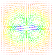
在本小节，我们将在二维域 $\Omega =\left(-1,1\right)\times \left(-1,1\right)$ 展示四个奇异点的演变过程，这些数值实例取自于 [16] [17] [18] [19] 等。参数为 $\lambda =v=\gamma =1$， $\epsilon =0.05$， $M=2$， $T=1$。初始速度为0，指向矢为 $d^0=\frac{\tilde{d}}{\sqrt{{\left|\tilde{d}\right|}^2+{\epsilon }^2}}$，其中， $\tilde{d}=\left(\frac{x^2}{a^2}+\frac{y^2}{b^2}-1,-xy\right)$， $a=0.5$， $b=0.25$。其指向场和速度场的演变过程如图1、图2所示。

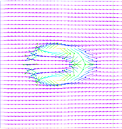(a) t = 0.001 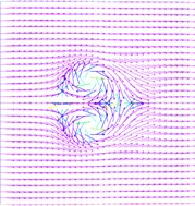(b) t = 0.02 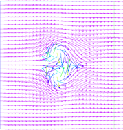(c) t = 0.05 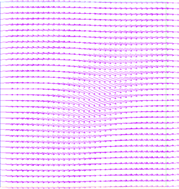(d) t = 0.1

Figure 1. The evolution of the director field of four singularities

图1. 四奇异点指向场的演变过程

(a) t = 0.005 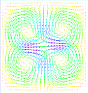(b) t = 0.05 (c) t = 0.1 (d) t = 0.3

Figure 2. The evolution of the director field of four singularities

图2. 四奇异点速度场的演变过程

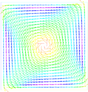
接下里来我们考虑旋转流，其初速度为 $u^0=\left(-\omega y,\omega x\right)$，其中， $\omega =50$，旋转流的湮没的指向场和速度场如图3、图4：

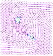(a) t = 0.05 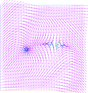(b) t = 0.1 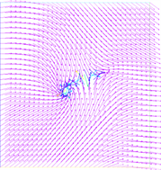(c) t = 0.2 (d) t = 0.3

Figure 3. The evolution of the director field of rotating flows

图3. 旋转流指向场的演变过程

(a) t = 0.001 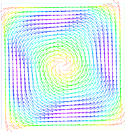(b) t = 0.01 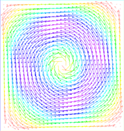(c) t = 0.1 (d) t = 0.2

Figure 4. The evolution of the director field of rotating flows

图4. 旋转流速度场的演变过程

4.2. 收敛阶

关于空间误差和收敛阶，我们仍取二维域 $\Omega =\left(-1,1\right)\times \left(-1,1\right)$，初值取 $u^0=0$， $d^0=\left(\sin \left(a\right),\cos \left(a\right)\right)$，其中， $a=2\pi \left(\cos \left(x\right)-\sin \left(y\right)\right)$，使用 $\left(P_2,P_2,P_1\right)$ 元，其余参数为 $\lambda =0.01$， $v=\gamma =1$， $\epsilon =0.05$， $M=2$， $T=0.1$， $\Delta t=0.002$，我们可以观察到随着空间步长h减小，误差越来越小，速度和指向矢的L²和H¹收敛阶分别趋于3和2，见表1、表2。

Table 1. Error of spatial convergence

表1. 空间误差

Table 2. Order of spatial convergence

表2. 空间收敛阶

Table 3. Error of time convergence

表3. 时间误差

Table 4. Order of time convergence

表4. 时间收敛阶

关于时间误差和收敛阶，计算域如上，初值取 $u^0=0$， $d^0=\left(\sin \left(a\right),\cos \left(a\right)\right)$，其中， $a=4\pi {\left(x^4+y^4\right)}^2$，使用 $\left(P_2,P_2,P_1\right)$ 元，其余参数为 $\lambda =0.001$， $v=0.1$， $\gamma =1$， $\epsilon =0.05$， $M=2$， $T=0.1$， $h=1/14$，可观察到随着时间步长 $\Delta t$ 减小，误差越来越小，指向矢的收敛阶优于速度的收敛阶，趋近于2，见表3、表4。

5. 结语

本文主要研究了一种基于Crank-Nicolson外推格式的二阶线性格式求解Ginzburg-Landau模型。然后，在离散情况下，证明了该格式是无条件能量稳定的。最后，通过数值实例展示了四个奇异点和旋转流的指向场和速度场的湮没过程，验证了该格式的二阶数值精度。

NOTES

^*通讯作者。