S-型分布时滞中立型神经网络稳定性
Stability of Neutral Neural Networks with S-Type Distributed Delays
DOI: 10.12677/PM.2022.124065, PDF, HTML, XML, 下载: 343  浏览: 1,924  科研立项经费支持
作者: 王 冰, 孙小淇:青岛大学,数学与统计学院,山东 青岛
关键词: S-型分布时滞中立型神经网络同胚映射Lyapunov-Krasovskii泛函S-type Distributed Delays Neutral Neural Networks Homeomorphic Mapping Lyapunov-Krasovskii Functional
摘要: 本文研究了一类具有S-型分布时滞的中立型神经网络的全局渐近稳定性问题。首先利用同胚映射理论证明系统平衡点的存在唯一性。然后构造Lyapunov-Krasovskii泛函,利用不等式方法得到新的稳定性代数判据。最后,通过两个数值例子并运用MATLAB仿真验证了新判据的有效性。
Abstract: In this paper, the global asymptotic stability of a class of neutral neural networks with S-type distributed delays is studied. Firstly, the existence and uniqueness of the equilibrium point of the system are proved by using the homeomorphic mapping theory. Secondly, by constructing an appropriate Lyapunov-Krasovskii functional and using the inequality method, a new algebraic criterion of stability is obtained. Finally, the effectiveness of the new criterion is proved by two numerical examples and MATLAB simulation.
文章引用:王冰, 孙小淇. S-型分布时滞中立型神经网络稳定性[J]. 理论数学, 2022, 12(4): 580-589. https://doi.org/10.12677/PM.2022.124065

1. 引言

近年来,人工神经网络在联想记忆、组合优化、图像处理等领域得到成功应用(见 [1] [2] [3] )。例如神经网络应用于联想记忆实质是:将要存储的记忆样本用矢量表示;神经网络在输入记忆样本后,经过演化最终稳定在记忆样本上;当神经网络的输入为非线性记忆样本时,网络输出应该要么稳定于记忆样本,要么稳定于稳定的非线性样本;不论外部输入为何,神经网络的输出应该是稳定的。用神经网络解决各种组合优化问题时的实质是把问题映射为一神经网络动力系统,并写出相应的能量函数表达式和动力学方程,他们应满足问题的约束条件;最后研究神经网络的动力学过程,以保证网络的稳态输出与能量函数的极小值和组合优化问题的解相对应。因此稳定性的分析一直是神经网络理论的研究重点。在实际应用中,神经网络的系统状态有时不仅依赖于神经元当前的状态,而且还与过去的状态即过去状态对时间的导数有关,这样的系统称为中立型神经网络。

目前,中立型神经网络在种群生态学、分布式网络、传播和扩散模型中得到了广泛的应用(见 [4] [5] [6] )。中立型神经网络的稳定性也得到充分发展(见 [7] - [13] )。2018年,G.B. Zhang等人在 [12] 中研究了一类具有混合时变时滞的中立型神经网络的鲁棒稳定性问题。通过构造多重Lyapunov-Krasovskii泛函,利用推广的基于多重Wirtinger的积分不等式得到了两个LMI形式的判据。相较于一重Lyapunov-Krasovskii泛函,进一步降低了条件的保守性。2020年,S. Arik在 [13] 中研究了一类具有多时滞的中立型神经网络的全局渐近稳定性问题。文章首先利用同胚映射理论证明了平衡点的存在唯一性。然后通过构造Lyapunov-Krasovskii泛函和利用矩阵不等式得到了与时滞无关的代数判据。

S-型时滞包含了离散时滞和连续时滞,最早由王林山教授和徐道义教授在 [14] 中提出。目前关于具有S-型分布时滞的神经网络稳定性得到广泛关注(见 [15] [16] [17] [18] [19] )。2011年,Y.F. Wang等人在 [18] 中研究了一类S-型分布时滞的高阶Hopfield型神经网络的全局指数稳定性问题。文章利用拓扑度理论和微分不等式技术,证明了平衡点的存在性和全局存在性。通过截距方程得到了全局指数稳定性的一些易于验证的充分条件,这些条件还具有更广泛的适应性。2018年,Q. Yao等人在 [19] 中研究了一类S-型分布式时滞的反应扩散随机Hopfield神经网络的指数稳定性问题。文章首先通过截距法将无限时滞问题转化为有限时滞问题。然后利用广义Halanay不等式研究了有限时滞网络的适定性,并用M函数讨论均方意义上的全局指数稳定性,最后借助逼近方法,得到了原始网络的适定性和稳定性。

但是据作者所知,目前关于S-型分布时滞的中立型神经网络稳定性研究较少,其原因是中立型时滞的引入,给这类神经网络的稳定性分析带来较大的困难。因此本文研究了具有S-型分布时滞的中立型神经网络的全局渐近稳定性问题,并得到了与时滞无关的易于验证的代数判据。

本文的结构安排如下:

第二节预备知识中给出S-型分布时滞中立型神经网络的具体形式,给出本文需要的两个引理;第三节主要结论包含两部分,第一部分通过同胚映射理论证明平衡点的存在唯一性,第二部分通过利用Lyapunov理论得到平衡点的全局渐近稳定性判据;第四节通过两个具体的数值例子并用MATLAB仿真验证了新判据的有效性;第五节结论是对全文的一个总结以及对未来的展望。

2. 预备知识

考虑如下具有S-型分布时滞的中立型神经网络系统:

{ x ˙ i ( t ) = c i x i ( t ) + j = 1 n a i j f j ( x j ( t ) ) + j = 1 n b i j g j ( 0 x j ( t + θ ) d η j ( θ ) ) + j = 1 n e i j x ˙ j ( t ξ i j ( t ) ) + u i , x i ( σ + θ ) = ϕ i ( θ ) , t σ 0 , θ 0 , i , j = 1 , 2 , , n , (1)

其中: x i ( t ) 表示第i个神经元的状态, c i 是正常数, u i 是外部输入。 f i ( ) g i ( ) 是非线性激活函数。 a i j b i j 表示神经元之间的连接权重。 ξ i j ( t ) 表示中立型时变时滞且 e i j 表示延迟状态的时间导数的系数。

η j ( θ ) ( , 0 ] 上的非减的有界变差函数且满足 0 d η j ( θ ) = γ j > 0 j = 1 , 2 , , n 0 x j ( t + θ ) d η j ( θ )

Lebesgue-Stieltjes可积的。

对于系统(1),假设下列条件成立:

(T1) f i ( ) g i ( ) 满足Lipschitz条件。即存在常数 l i > 0 s i > 0 ,对所有 x , y R

| f i ( x ) f i ( y ) | l i | x y | | g i ( x ) g i ( y ) | s i | x y | i = 1 , 2 , , n

(T2)中立型时变时滞 ξ i j ( t ) 满足 0 ξ i j ( t ) ξ ξ 是常数且 ξ ˙ i j ( t ) ξ ¯ 0 ξ ¯ < 1

引理2.1 [13] 如果映射 H ( x ) C 0 ,满足对任意的x和y,当 x y 时有 H ( x ) H ( y ) ,且当 x 时有 H ( x ) ,那么 H ( x ) 是一个同胚映射。

引理2.2 [16] 若 f ( t , θ ) f t ( t , θ ) = d d t f ( t , θ ) t [ a , b ] θ ( , 0 ] 时连续, η ( θ ) ( , 0 ] 上的有界不减变差函数,且 0 d η ( θ ) = k < ,则

d d t 0 f ( t , θ ) d η ( θ ) = 0 d d t f ( t , θ ) d η j ( θ )

3. 主要结论

3.1. 平衡点的存在唯一性

定理3.1 对于中立型神经网络(1),如果存在正常数 r 1 , r 2 , , r n 0 < α < 1 使得下列条件成立

(T3) μ i = r i c i 1 + α 1 α l i j = 1 n r j | a j i | 1 + α 1 α s i γ i j = 1 n r j | b j i | > 0

ν i j = α n r j ( 1 ξ ¯ ) ( 1 + α ) r i | e i j | > 0 i , j = 1 , 2 , , n

且还满足假设(T1) (T2),则系统(1)存在唯一的平衡点。

证明:若 x * = ( x 1 * , x 2 * , , x n * ) T 是系统(1)的一个平衡点,则 x * 满足下式

c i x i * + j = 1 n a i j f j ( x j * ) + j = 1 n b i j g j ( γ j x j * ) + u i = 0

定义映射 H ( x ) = ( h 1 ( x ) , h 2 ( x ) , , h n ( x ) ) ,其中

h i ( x ) = c i x i + j = 1 n a i j f j ( x j ) + j = 1 n b i j g j ( γ j x j ) + u i i = 1 , 2 , , n

对于 x , y R n x y ,由条件(T1)可得

i = 1 n r i sgn ( x i y i ) ( h i ( x ) h i ( y ) ) = i = 1 n r i c i sgn ( x i y i ) ( x i y i ) + i = 1 n j = 1 n r i a i j sgn ( x i y i ) ( f j ( x j ) f j ( y j ) ) + i = 1 n j = 1 n r i b i j sgn ( x i y i ) ( g j ( γ j x j ) g j ( γ j y j ) ) i = 1 n r i c i | x i y i | + i = 1 n j = 1 n r i | a i j | | f j ( x j ) f j ( y j ) | + i = 1 n j = 1 n r i | b i j | | g j ( γ j x j ) g j ( γ j y j ) | i = 1 n r i c i | x i y i | + i = 1 n j = 1 n l i r j | a j i | | x i y i | + i = 1 n j = 1 n s i γ i r j | b j i | | x i y i | (2)

此外,显然下面不等式是成立的

α n i = 1 n j = 1 n ( r j c j | x j y j | ( 1 ξ ¯ ) r j c j | x j y j | ) + i = 1 n j = 1 n r j c j | e i j | | x j y j | 0 (3)

将(3)式加到(2)式的右端,可得

i = 1 n r i sgn ( x i y i ) ( h i ( x ) h i ( y ) ) ( 1 α ) i = 1 n ( r i c i 1 + α 1 α l i j = 1 n r j | a j i | 1 + α 1 α s i γ i j = 1 n r j | b j i | ) | x i y i | i = 1 n j = 1 n ( α n r j ( 1 ξ ¯ ) ( 1 + α ) r i | e i j | ) c j | x j y j | = ( 1 α ) i = 1 n μ i | x i y i | i = 1 n j = 1 n ν i j c j | x j y j | (4)

由条件(T3)可得

i = 1 n r i sgn ( x i y i ) ( h i ( x ) h i ( y ) ) ( 1 α ) i = 1 n μ i | x i y i | ( 1 α ) μ m i = 1 n | x i y i | = ( 1 α ) μ m x y 1 (5)

其中 μ m = min { u i } , i = 1 , 2 , , n

对(5)式两端同取绝对值可得

| i = 1 n r i sgn ( x i y i ) ( h i ( x ) h i ( y ) ) | ( 1 α ) μ m x y 1 i = 1 n r i | sgn ( x i y i ) | | ( h i ( x ) h i ( y ) ) | ( 1 α ) μ m x y 1 R M H ( x ) H ( y ) 1 ( 1 α ) μ m x y 1 (6)

其中 R M = max { r i } , i = 1 , 2 , , n

y = 0 ,则由三角不等式可得

H ( x ) 1 ( 1 α ) μ m R M x 1 + H ( 0 ) 1 (7)

从(6)式可知若 x y H ( x ) H ( y ) 。在这里 x = x 1 ,因此从(7)式可知当 x 时有 H ( x ) ,由引理2.1可知 H ( x ) 是同胚映射。因此系统(1)存在唯一平衡点。

3.2. 平衡点的全局渐近稳定性

由定理3.1可知系统(1)存在唯一的平衡点 x * ,作变换 y i ( t ) = x i ( t ) x i * ,则系统(1)等价于如下系统

{ y ˙ i ( t ) = c i y i ( t ) + j = 1 n a i j p j ( y j ( t ) ) + j = 1 n b i j q j ( 0 y j ( t + θ ) d η j ( θ ) ) + j = 1 n e i j y ˙ j ( t ξ i j ( t ) ) , y i ( σ + θ ) = Φ i ( θ ) , t σ 0 , θ 0 , i , j = 1 , 2 , , n , (8)

其中

Φ i ( θ ) = ϕ i ( θ ) x i * , p j ( y j ( t ) ) = f j ( y j ( t ) + x j * ) f j ( x j * ) , q j ( 0 y j ( t + θ ) d η j ( θ ) ) = g j ( 0 ( y j ( t + θ ) + x j * ) d η j ( θ ) ) g j ( 0 x j * d η j ( θ ) ) .

由条件(T1)可得下面条件是成立的

(T4) | p j ( y j ( t ) ) | l j | y j ( t ) | | q j ( 0 y j ( t + θ ) d η j ( θ ) ) | s j | 0 y j ( t + θ ) d η j ( θ ) |

定理3.2 若系统(8)满足条件(T2),(T3)和(T4),则系统(8)的平衡点是全局渐近稳定的。

证明:对 t 0 ,构造如下Lyapunov-Krasovskii泛函

V ( t ) = V 1 ( t ) + V 2 ( t ) V 1 ( t ) = i = 1 n β r i | y i ( t ) | + ( 1 sgn 2 ( y i ( t ) ) ) i = 1 n j = 1 n | b i j | s j 0 ( t + θ t | y j ( s ) | d s ) d η j ( θ ) V 2 ( t ) = β α n i = 1 n j = 1 n r j t ξ i j ( t ) t | y ˙ j ( s ) | d s + β ( 1 + α ) i = 1 n j = 1 n r i s j | b i j | 0 ( t + θ t | y j ( s ) | d s ) d η j ( θ ) + λ i = 1 n j = 1 n t + θ t | y j ( s ) | d s

先考虑 V 1 ( t ) ,分三种情况考虑

y i ( t ) = 0 时,则 sgn ( y i ( t ) ) = 0 ,那么

V 1 ( t ) = i = 1 n β r i | y i ( t ) | + i = 1 n j = 1 n | b i j | s j 0 ( t + θ t | y j ( s ) | d s ) d η j ( θ )

V 1 ( t ) 关于时间t求导可得

V ˙ 1 ( t ) = i = 1 n y ˙ i ( t ) + i = 1 n j = 1 n | b i j | s j ( 0 | y j ( t ) | d η j ( θ ) 0 | y j ( t + θ ) | d η j ( θ ) ) i = 1 n β r i sgn ( y i ( t ) ) y ˙ i ( t ) + j = 1 n j = 1 n | a i j | l j | y j ( t ) | + i = 1 n j = 1 n | b i j | s j γ j | y j ( t ) | + i = 1 n j = 1 n | e i j | | y ˙ j ( t ξ i j ( t ) ) |

y i ( t ) > 0 时,则 sgn ( y i ( t ) ) = 1 ,那么 V 1 ( t ) = i = 1 n β r i sgn ( y i ( t ) ) y i ( t ) ,对 V 1 ( t ) 关于时间t求导可得

V ˙ 1 ( t ) = i = 1 n β r i sgn ( y i ( t ) ) y ˙ i ( t ) i = 1 n β r i sgn ( y i ( t ) ) y ˙ i ( t ) + j = 1 n j = 1 n | a i j | l j | y j ( t ) | + i = 1 n j = 1 n | b i j | s j γ j | y j ( t ) | + i = 1 n j = 1 n | e i j | | y ˙ j ( t ξ i j ( t ) ) |

y i ( t ) < 0 时,则 sgn ( y i ( t ) ) = 1 ,那么 V 1 ( t ) = i = 1 n β r i sgn ( y i ( t ) ) y i ( t ) ,对 V 1 ( t ) 关于时间t求导可得

V ˙ 1 ( t ) = i = 1 n β r i sgn ( y i ( t ) ) y ˙ i ( t ) i = 1 n β r i sgn ( y i ( t ) ) y ˙ i ( t ) + j = 1 n j = 1 n | a i j | l j | y j ( t ) | + i = 1 n j = 1 n | b i j | s j γ j | y j ( t ) | + i = 1 n j = 1 n | e i j | | y ˙ j ( t ξ i j ( t ) ) |

综上可得

V ˙ 1 ( t ) i = 1 n β r i sgn ( y i ( t ) ) y ˙ i ( t ) + δ 1 ( t ) + δ 2 ( t ) + δ 3 ( t ) (9)

其中

δ 1 ( t ) = j = 1 n j = 1 n | a i j | l j | y j ( t ) | , δ 2 ( t ) = i = 1 n j = 1 n | b i j | s j γ j | y j ( t ) | , δ 3 ( t ) = i = 1 n j = 1 n | e i j | | y ˙ j ( t ξ i j ( t ) ) |

再对 V 2 ( t ) 关于时间t求导可得

V ˙ 2 ( t ) = β α n i = 1 n j = 1 n r j | y ˙ j ( t ) | β α n i = 1 n j = 1 n r j ( 1 ξ ˙ i j ( t ) ) | y ˙ j ( t ξ i j ( t ) ) | + β ( 1 + α ) i = 1 n j = 1 n r i s j | b i j | ( 0 | y j ( t ) | d η j ( θ ) 0 | y j ( t + θ ) | d η j ( θ ) ) + λ i = 1 n j = 1 n | y j ( t ) | λ i = 1 n j = 1 n | y j ( t + θ ) | (10)

由(9)式和(10)式可得

V ˙ ( t ) β i = 1 n r i ρ i ( t ) y ˙ i ( t ) β α n i = 1 n j = 1 n r j ( 1 ξ ˙ i j ( t ) ) | y ˙ j ( t ξ i j ( t ) ) | + β ( 1 + α ) i = 1 n j = 1 n r i s j | b i j | ( 0 | y j ( t ) | d η j ( θ ) 0 | y j ( t + θ ) | d η j ( θ ) ) + λ i = 1 n j = 1 n | y j ( t ) | λ i = 1 n j = 1 n | y j ( t + θ ) | + δ 1 ( t ) + δ 2 ( t ) + δ 3 ( t ) (11)

其中 ρ i ( t ) = sgn ( y i ( t ) ) + α sgn ( y ˙ i ( t ) )

因为 0 < α < 1 ,若 y i ( t ) > 0 ,则 ρ i ( t ) = 1 + α sgn ( y ˙ i ( t ) ) > 0 。若 y i ( t ) = 0 ,则 ρ i ( t ) = 0

y i ( t ) < 0 ,则 ρ i ( t ) = 1 + α sgn ( y ˙ i ( t ) ) < 0 ,所以 ρ i ( t ) y i ( t ) = | ρ i ( t ) | | y i ( t ) |

很容易得到 min { | ρ i ( t ) | } = 1 α max { | ρ i ( t ) | } = 1 + α i = 1 , 2 , , n

将(8)式代入(11)式化简可得

V ˙ ( t ) β ( 1 α ) i = 1 n r i c i | y i ( t ) | + β ( 1 + α ) i = 1 n j = 1 n r i | a i j | | p j ( y j ( t ) ) | + β ( 1 + α ) i = 1 n j = 1 n r i s j | b i j | 0 | y j ( t ) | d η j ( θ ) + β ( 1 + α ) i = 1 n j = 1 n r i | e i j | | y ˙ j ( t ξ i j ( t ) ) | β α n i = 1 n j = 1 n r j ( 1 ξ ¯ ) | y ˙ j ( t ξ i j ( t ) ) | + λ i = 1 n j = 1 n | y j ( t ) | λ i = 1 n j = 1 n | y j ( t + θ ) | + δ 1 ( t ) + δ 2 ( t ) + δ 3 ( t ) (12)

由条件(T3)可得

V ˙ ( t ) β ( 1 α ) i = 1 n μ i | y i ( t ) | β i = 1 n j = 1 n ν i j | y ˙ j ( t ξ i j ( t ) ) | + n λ i = 1 n y i ( t ) + δ 1 ( t ) + δ 2 ( t ) + δ 3 ( t ) β ( 1 α ) μ m y ( t ) 1 β ν m i = 1 n j = 1 n | y ˙ j ( t ξ i j ( t ) ) | + n λ y ( t ) 1 + l M A 1 y ( t ) 1 + s M γ M B 1 y ( t ) 1 + e M i = 1 n j = 1 n | y ˙ j ( t ξ i j ( t ) ) | (13)

其中 μ m = min { μ i } ν m = min { ν i j } l M = max { l i } s M = max { s i } γ M = max { γ i } e M = max { e i j } i , j = 1 , 2 , , n

选取 β = n λ + l M A 1 + s M γ M B 1 μ m ( 1 α ) + e M ν m ,则由(13)式可得

V ˙ ( t ) ( 1 α ) μ m e M ν m y ( t ) 1 ν m ( n λ + l M A 1 + s M γ M B 1 ) μ m ( 1 α ) i = 1 n j = 1 n | y ˙ j ( t ξ i j ( t ) ) | (14)

显然对任意的i和j,若 y i ( t ) 0 y ˙ j ( t ξ i j ( t ) ) 0 ,则 V ˙ ( t ) < 0 恒成立。若 y i ( t ) = 0

y ˙ j ( t ξ i j ( t ) ) = 0 ,则由(12)式可知, V ˙ ( t ) λ i = 1 n j = 1 n | y j ( t + θ ) | ,所以当 y j ( t + θ ) 0 V ˙ ( t ) < 0 成立。当

y i ( t ) = 0 y ˙ j ( t ξ i j ( t ) ) = 0 y j ( t + θ ) = 0 时, V ˙ ( t ) = 0 。因此除了平衡点之外, V ˙ ( t ) < 0 恒成立。

由Lyapunov稳定性理论可知,系统(8)的平衡点是渐近稳定的。可以看出,用于稳定性分析的Lyapunov-Krasovskii泛函是径向无界的,即当 y ( t ) V ( t ) ,说明 y ( t ) = 0 是全局渐近稳定的。

4. 数值实验

对于S-型分布时滞中立型神经网络(1),假设满足下列条件

A = 1 5 [ 2 2 1 1 1 2 2 1 2 2 2 1 1 1 2 1 ] B = [ 2 2 1 1 2 1 2 1 1 1 2 2 2 1 1 2 ] E = 1 25 [ 1 1 1 1 1 1 1 1 1 1 1 1 1 1 1 1 ]

f i ( x ) = 0.6 tanh ( x ) g i ( x ) = 0.4 tanh ( x ) c i = 5 u i = 0.5 ξ i j ( t ) = 0.5 i , j = 1 , 2 , , n 。令 α = 0.5 ,取 r 1 = r 2 = r 3 = r 4 = 1

例4.1 对于非减有界变差函数 η j ( θ ) ,当取

η j ( θ ) = { 1 , θ τ j 0 , τ j θ 0 时,

0 d η j ( θ ) = 1 ,并且 g j ( 0 x j ( t + θ ) d η j ( θ ) ) = g j ( x j ( t τ j ) ) j = 1 , 2 , , n 。若取 τ j = 0.5 j = 1 , 2 , , n ,则满足定理3.2的条件,因此平衡点是全局渐近稳定的,其神经元的状态轨迹见图1

例4.2 当 η j ( θ ) 连续可微且 η j ( θ ) = γ j ( θ ) j = 1 , 2 , , n 时,则

g j ( 0 x j ( t + θ ) d η j ( θ ) ) = g j ( 0 γ j ( s ) x j ( t s ) d s ) j = 1 , 2 , , n

若取 η j ( θ ) = e θ j = 1 , 2 , , n ,则满足定理3.2的条件,因此平衡点是全局渐近稳定的,其神经元的状态轨迹见图2

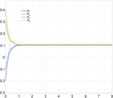
Figure 1. The neurons states trajectory of Example 4.1

图1. 例4.1神经元的状态轨迹

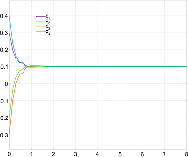
Figure 2. The neurons states trajectory of Example 4.2

图2. 例4.2神经元的状态轨迹

5. 结论

S-型分布时滞包含了离散时滞和连续时滞,因此研究S-型分布时滞神经网络的动力学行为在实际应用和理论上都有重要意义。本文研究了一类具有S-型分布时滞的中立型神经网络的全局渐近稳定性问题。通过利用同胚映射理论、不等式技巧和构建合适的Lyapunov-Krasovskii泛函,得到了与时滞参数无关的稳定性代数判据,相较于LMI形式的判据,该判据更易得到验证。

因为神经递质释放的信号可能在时间上具有随机波动,所以随机扰动在神经元中的电位传播中是不可避免的。因此在未来的研究中,作者想进一步考虑带有随机项的S-型分布时滞中立型神经网络的稳定性问题。

基金项目

山东省自然科学基金项目(编号ZR2019PA00)资助。

参考文献

[1] Tamura, H., Zhang, Z., Xu, X.S., Ishii, M. and Tang, Z. (2005) Lagrangian Object Relaxation Neural Network for Combinatorial Optimization Problems. Neurocomputing, 68, 297-305.
https://doi.org/10.1016/j.neucom.2005.03.003
[2] Calabuig, D., Monserrat, J.F., Gmez-Barquero, D. and Lzaro, O. (2008) An Efficient Dynamic Resource Allocation Algorithm for Packet-Switched Communication Networks Based on Hopfield Neural Excitation Method Original Research Article. Neurocomputing, 71, 3439-3446.
https://doi.org/10.1016/j.neucom.2007.10.009
[3] Sammouda, R., Adgaba, N., Touir, A. and Al-Ghamdi, A. (2014) Agriculture Satellite Image Segmentation Using a Modified Artificial Hopfield Neural Network Original Research Article. Computers in Human Behavior, 30, 436-441.
https://doi.org/10.1016/j.chb.2013.06.025
[4] Kolmanovskii, V.B. and Nosov, V.R. (1986) Stability of Functional Differential Equations. Elsevier, London.
[5] Kuang, Y. (1993) Delay Differential Equations: With Applications in Population Dynamics. Elsevier, Boston.
[6] Niculescu, S.I. (2001) Delay Effects Stability: A Robust Control Approach. Springer, Berlin.
[7] Pauwels, R., Peng, W.L., Wu, Q.X. and Zhang, Z.Q. (2016) LMI-Based Global Ex-ponential Stability of Equilibrium Point for Neutral Delayed BAM Neural Networks with Delays in Leakage Terms via New Inequality Technique. Neurocomputing, 199, 103-113.
https://doi.org/10.1016/j.neucom.2016.03.030
[8] Samli, R., Senan, S., Yucel, E. and Orman, Z. (2019) Some Generalized Global Stability Criteria for Delayed Cohen-Grossberg Neural Networks of Neutral-Type. Neural Networks, 116, 198-207.
https://doi.org/10.1016/j.neunet.2019.04.023
[9] Faydasicok, O. (2020) New Criteria for Global Stability of Neutral-Type Cohen-Grossberg Neural Networks with Multiple Delays. Neural Networks, 125, 330-337.
https://doi.org/10.1016/j.neunet.2020.02.020
[10] Popa, C.A. (2020) Global μ-Stability of Neutral-Type Impulsive Complex-Valued BAM Neural Networks with Leakage Delay and Unbounded Time-Varying Delays. Neurocomputing, 376, 73-94.
https://doi.org/10.1016/j.neucom.2019.09.008
[11] Wan, L. and Zhou, Q.H. (2021) Exponential Stability of Neu-tral-Type Cohen-Grossberg Neural Networks with Multiple Time-Varying Delays. IEEE Access, 9, 48914-48922.
https://doi.org/10.1109/ACCESS.2021.3068191
[12] Zhang, G.B., Wang, T., Li, T. and Fei, S.M. (2018) Multiple Integral Lyapunov Approach to Mixed-Delay-Dependent Stability of Neutral Neural Networks. Neurocomputing, 275, 1782-1792.
https://doi.org/10.1016/j.neucom.2017.10.021
[13] Arik, S. (2020) New Criteria for Stability of Neutral-Type Neural Networks with Multiple Time Delays. IEEE Transactions on Neural Networks and Learning Systems, 31, 1504-1513.
https://doi.org/10.1109/TNNLS.2019.2920672
[14] Wang, L.S. and Xu, D.Y. (2002) Global Asymp-totic Stability of Bidirectional Associative Memory Neural Networks with S-Type Distributed Delays. International Journal of System Science, 33, 869-877.
https://doi.org/10.1080/00207720210161777
[15] Liu, P.C., Yi, F.Q., Guo, Q., Yang, J. and Wu, W. (2008) Analysis on Global Exponential Robust Stability of Reaction-Diffusion Neural Networks with S-Type Distributed De-lays. Physica D, 237, 475-485.
https://doi.org/10.1016/j.physd.2007.09.014
[16] Zhang, R.J. and Wang, L.S. (2009) Global Exponential Robust Stability of Interval Cellular Neural Networks with S-Type Distributed Delays. Mathematical and Computer Modelling, 50, 380-385.
https://doi.org/10.1016/j.mcm.2009.04.016
[17] Huang, Z.K., Li, X.Z., Mohamad, S. and Lu, Z.Y. (2009) Robust Stability Analysis of Static Neural Network with S-Type Distributed Delays. Applied Mathematical Modelling, 33, 760-769.
https://doi.org/10.1016/j.apm.2007.12.006
[18] Wang, Y.F., Lu, C.G., Ji, G.R. and Wang, L.S. (2011) Global Exponential Stability of High-Order Hopfield-Type Neural Networks with S-Type Distributed Time Delays. Communications in Nonlinear Science and Numerical Simulation, 16, 3319-3325.
https://doi.org/10.1016/j.cnsns.2010.11.005
[19] Yao, Q., Wang, L.S. and Wang, Y.F. (2018) Exist-ence-Uniqueness and Stability of Reaction-Diffusion Stochastic Hopfield Neural Networks with S-Type Distributed Time Delays. Neurocomputing, 275, 470-477.
https://doi.org/10.1016/j.neucom.2017.08.060