基于动态虚拟相机的旋转棱镜扫描成像系统运动模糊消除技术研究
Motion Deblurring Technology Research for Risley Prism Scanning Imaging System Based on Dynamic Virtual Camera
DOI: 10.12677/MOS.2023.123251, PDF, HTML, XML, 下载: 189  浏览: 384  国家自然科学基金支持
作者: 李新东*, 李安虎#, 周正旸, 刘兴盛, 邓兆军:同济大学机械与能源工程学院,上海
关键词: 运动模糊消除旋转棱镜动态虚拟相机Motion Deblurring Risley Prism Dynamic Virtual Camera
摘要: 旋转棱镜–相机成像系统在动态目标识别和跟踪等新兴领域展现了很好的应用前景。然而,其性能受到运动模糊问题的限制。为了解决旋转棱镜–相机成像系统中的运动模糊问题,本文基于运动成像分析方法,建立了动态虚拟相机的运动模糊数学模型,以表征系统的实时成像模糊机制。通过分析动态虚拟相机一阶运动表达式,提出了动态虚拟相机成像的运动模糊核估计方法和运动模糊消除算法。基于所提出的方法,可以获得扫描图像的运动模糊核,然后结合维纳滤波来消除模糊。实验结果表明,所提出的运动模糊消除算法能有效地消除运动模糊,提高实时扫描成像系统的成像质量。
Abstract: The Rotating Prism-Camera Imaging System (RPCIS) demonstrates promising application prospects in the emerging field of dynamic target tracking and recognition. However, its performance is lim-ited by motion blur issues. To solve the motion blur problem in the rotating prism-camera imaging system, developed by motion imaging analysis methods, a motion blurring mathematical model of the dynamic virtual camera (DVC) is established to characterize the real-time imaging blurring mechanism. By analyzing the kinematics of DVC based on first-order motion expression of rotating double-prism scanners, a motion blur kernel estimation method and the algorithm for motion deblurring are proposed. Based on the proposed method, the motion blur kernel of the scanning image can be obtained, and then the wiener filtering is combined to eliminate the blur. Experi-mental results demonstrate that the proposed motion deblurring method effectively eliminates motion blur and improves the image quality of the real-time scanning imaging system.
文章引用:李新东, 李安虎, 周正旸, 刘兴盛, 邓兆军. 基于动态虚拟相机的旋转棱镜扫描成像系统运动模糊消除技术研究[J]. 建模与仿真, 2023, 12(3): 2740-2751. https://doi.org/10.12677/MOS.2023.123251

1. 引言

为了满足各种搜索和跟踪需求,研究人员提出并发展了各种成像系统来实现搜索和跟踪成像 [1] 。这些设备通常使用面阵相机或线扫描相机,并采用基于镜面反射的扫描成像或基于棱镜折射的扫描成像两种扫描方式 [2] [3] 。这些系统旨在实现全景扫描成像,并在搜索后跟踪目标 [4] - [10] 。

旋转棱镜扫描仪因其紧凑结构、低转动惯量和良好的指向性能,已被广泛应用于激光通信、激光雷达和光束扫描等领域 [11] [12] [13] [14] [15] 。通过在相机前安装旋转棱镜,可以精确地改变相机的视轴指向。Lavigne等人利用旋转棱镜构建了一套步进–凝视成像系统,实现了高分辨率和大视场成像 [16] 。基于类似原理,旋转棱镜被用于图像拼接、超分辨率、多视角成像、三维重建和目标跟踪 [14] - [24] 。

对于旋转棱镜扫描仪,先前的研究主要关注动态扫描模式和光束畸变。Marshall等人通系统地研究了旋转棱镜扫描模式,分析了不同旋转速度、不同棱镜楔角下的光束扫描图案 [25] 。Jeno等人探讨了具有任意数量棱镜的棱镜组的扫描轨迹 [26] 。Schwarze等人发现了棱镜光束压缩效应,提出光束压缩系数与出射光和出射面法向量夹角的余弦值成反比 [27] 。Lavigne等人指出旋转棱镜的成像畸变与棱镜形状相似,发现图像畸变的大小可以近似为线性变形 [28] 。Huang等人提出了一种误差源检测方法,用迭代算法消除图像矫正误差 [29] 。之前的这些研究主要集中在静态成像上,很少涉及动态成像,在扫描成像过程中,棱镜是旋转的,这种模式可以看作是相机在动态连续地扫描场景,所以需要考虑运动补偿 [30] [31] 。

在扫描成像应用中,相机曝光时间内被成像物体与相机成像平面之间存在相对运动,这会导致运动模糊和图像退化。因此,研究运动模糊消除技术对解决这个问题至关重要。为此,我们基于旋转棱镜相机成像系统提出了动态虚拟相机成像模型,并基于动态虚拟相机模型进行运动学分析,提出了一种扫描图像运动模糊消除算法,提高了系统成像清晰度。

2. 基于动态虚拟相机模型的运动分析

图1所示,旋转双棱镜–相机成像系统由一个相机以及一对共轴但是独立旋转的旋转棱镜组成,且相机的光心一般布置在光轴上。通过两个棱镜的独立旋转,相机的视轴可以被调整到一个特定的区域从而改变相机的成像视场,视轴调整后的具体指向取决于两个棱镜的转角。基于这个原理我们提出了一个等效的虚拟相机模型,这个模型可以生动地描述旋转棱镜–相机成像系统的成像特性,如图1所示,旋转棱镜–相机成像系统在特定棱镜角度组合下拍摄的任何图像都可以被视为虚拟相机拍摄的图像。在本节中,我们将进一步探讨虚拟相机的位姿计算方法并对虚拟相机进行运动学分析。

Figure 1. Schematic diagram of the model of the dynamic virtual camera

图1. 动态虚拟相机模型示意图

2.1. 虚拟相机位姿计算

图1中,A0、A1、A2、A3和A4分别定义为实际相机的视轴方向向量、棱镜1入射面的折射光向量、棱镜1的出射光向量、棱镜2入射面的折射光向量、棱镜2的出射光向量。根据折射定律 [12] ,折射光束可以表示为:

A o u t = n 1 n 2 A i n + ( 1 ( n 1 n 2 ) 2 [ 1 ( A i n N i ) 2 ] n 1 n 2 ( A i n N i ) ) N i (1)

其中Ain和Aout分别是入射光束和折射光束的单位方向向量;Ni是棱镜工作面的单位法向量;n1和n2分别是入射介质和折射介质的折射率。对于空气,其折射率为1,旋转棱镜的折射率为n。

图1中,沿Zc正轴的四个平面的单位法向量依次表示为N1~N4

N 1 = [ x N 1 , y N 1 , z N 1 ] T = [ 0 , 0 , 1 ] T (2a)

N 2 = [ x N 2 , y N 2 , z N 2 ] T = [ cos ( θ 1 ) sin ( α ) , sin ( θ 1 ) sin ( α ) , cos ( α ) ] T (2b)

N 3 = [ x N 3 , y N 3 , z N 3 ] T = [ cos ( θ 2 ) sin ( α ) , sin ( θ 2 ) sin ( α ) , cos ( α ) ] T (2c)

N 4 = [ x N 4 , y N 4 , z N 4 ] T = [ 0 , 0 , 1 ] T (2d)

根据公式(1)和公式(2),可以得到出射光束矢量A4的表达式。

图1所示,定义俯仰角ρ为出射光束A4与Zp轴的正方向之间的夹角;方位角φ是出射光束在XLOLYL平面的投影与XL轴的正方向之间的夹角,假设 A 4 = [ x a 4 , y a 4 , z a 4 ] T ,则有:

ρ = arccos ( z a 4 ) (3a)

φ = { arccos ( x a 4 x a 4 2 + y a 4 2 ) y a 4 0 2 π arccos ( x a 4 x a 4 2 + y a 4 2 ) y a 4 < 0 (3b)

假设实际相机成像平面上两个像素点在图像坐标系中位置为(xs1,ys1)和(xs2,ys2),f是相机的焦距,则这两个像素点在相机坐标系中的坐标分别为(xs1,ys1,f)和(xs2,ys2,f)。由于相机光学中心作为相机坐标系的原点,我们可以得到两个入射光矢量 [ x s 1 , y s 1 , f ] T [ x s 2 , y s 2 , f ] T 。通过公式(1)~公式(3),我们可以计算得到图2中S1、S2、K1、K2。如图2所示,我们可以通过计算两个成像光束 S 1 = [ a 1 , b 1 , c 1 ] T S 2 = [ a 2 , b 2 , c 2 ] T 的交点得到虚拟相机的光学中心位置,定义为Ovc (xvcyvczvc),两个成像光束S1S2分别通过棱镜2表面Σ4上的出射点K1 (x1y1z1),K2 (x2y2z2)。

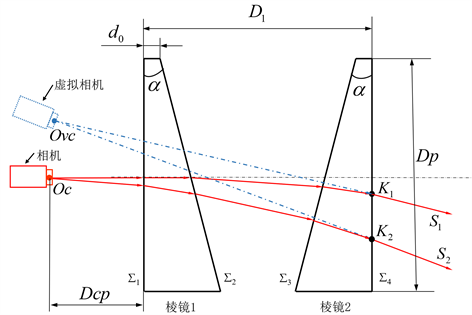
Figure 2. Schematic diagram of dynamic virtual camera pose computation

图2. 动态虚拟相机位姿计算原理图

通过计算以下公式得到动态虚拟相机的光学中心位置在实际相机坐标系中的位置:

{ x vc x 1 a 1 = y vc y 1 b 1 = z vc z 1 c 1 x vc x 2 a 2 = y vc y 2 b 2 = z vc z 2 c 2 (4)

基于公式(4)可以获得虚拟相机的光心Ovc与实际相机光心之间的平移矩阵 T v c = [ x v c , y v c , z v c ] T

虚拟相机与实际相机的相对旋转矩阵Rvc为实际相机视轴到出射光束之间的旋转矩阵,可以根据Rodrigues公式 [32] 求取。

虚拟相机在实际相机坐标系中的位姿可以表示为:

D V C R T = [ R v c T v c 0 1 ] (5)

基于公式(5),空间中任意一点在世界坐标系中的坐标与在虚拟相机像素坐标系的坐标之间的转换关系为:

[ u v v v 1 ] = 1 z v c [ f γ 0 0 0 f 0 0 0 0 0 1 ] [ R v c T v c 0 T 1 ] [ R w c T w c 0 T 1 ] [ x w y w z w 1 ] (6)

其中f是相机的焦距,γ是x和y像素轴之间的倾斜系数,Rwc和Twc分别是实际相机坐标系和世界坐标系之间的相对旋转矩阵和平移矩阵,实际相机的内部参数和外部参数可以通过张正友标定法得到。

2.2. 动态虚拟相机运动学分析

虽然虚拟相机的运动与棱镜的旋转之间的关系是非线性的,但虚拟相机的光学中心总是在相机视轴出射光束A4的反向延长线上,所以首先我们需要将棱镜的旋转速度映射到相机视轴出射光束A4的运动速度上。为了减少计算的复杂性,将采用一阶近似算法 [33] :该算法将棱镜看作是一个具有小顶角的光楔,其对光束的偏转角的大小只取决于棱镜的楔角和折射率,出射的光束指向棱镜主截面的厚端。如图3所示,光束在(O)处进入双棱镜系统并从棱镜1处射出。随着棱镜的旋转,偏转矢量δ1的末端沿着半径为δ1的圆π1移动。然后光束入射到棱镜2上,偏转矢量δ2的末端将沿着半径为δ2的圆运动。最后总的偏转矢量δ可以被认为是δ1和δ2的矢量和。

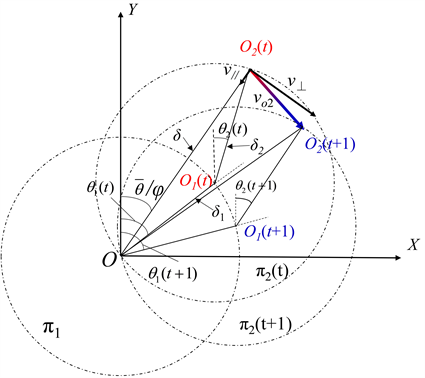
Figure 3. The kinematics analysis of the dynamic virtual camera based on a first-order centering algorithm

图3. 基于一阶近似算法的动态虚拟相机运动学分析

当两个棱镜的参数相同时,我们可以得到成像光轴方位角的一阶近似值,它相当于图4中棱镜扫描仪的等效主截面的旋转角度,其旋转角的表达式为:

θ ¯ = 1 2 ( θ 1 + θ 2 ) (7a)

棱镜之间的旋转角度差为:

θ ^ = θ 2 θ 1 (7b)

在一阶近似算法中, θ ¯ φ 之间的关系为:

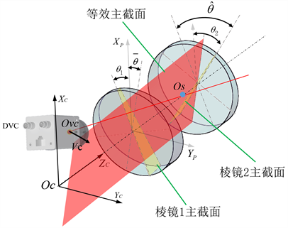
Figure 4. Schematic diagram of dynamic virtual camera equivalent main section

图4. 动态虚拟相机等效主截面的示意图

θ ¯ = φ (7c)

对于旋转双棱镜扫描成像系统,出射光束的偏转角为:

| δ | 2 = | δ 1 | 2 + | δ 2 | 2 2 | δ 1 | | δ 2 | cos ( π θ ^ ) , | δ | > 0 (8a)

两个棱镜的参数是相同的,因此它们具有相同的偏转角,所以:

δ 1 = δ 2 = n α (8b)

可以得到:

| δ | = 2 n α ( 1+ cos ( θ ^ ) ) 1 2 (8c)

O2的速度vo2可以分为沿δ的径向速度v和沿δ方向的法向速度v//

v = d θ ¯ d t = 1 2 ( ω 1 + ω 2 ) (9a)

v / / = d δ d t = 2 n α ( ω 2 ω 1 ) sin ( θ ^ ) ( 1 + cos ( θ ^ ) ) 1 2 (9b)

O2的速度为:

v O 2 = v + v / / (10a)

vo2的方向为:

{ β = θ ¯ + π 2 arctan ( v / / v ) v 0 β = θ ¯ π 2 arctan ( v / / v ) v < 0 (10b)

因此,基于一阶运动表达式,我们可以得到视轴指向方位角和俯仰角的变化方程,它同时也描述了动态虚拟相机所在光束的空间运动变化状态。

3. 运动模糊核估计方法及运动模糊消除算法

3.1. 运动模糊核估计

在扫描成像过程中动态虚拟相机与被成像物体之间产生相对运动,引入运动模糊并导致图像退化,运动模糊的图像退化表达方式为:

g ( u , v ) = f ( u , v ) h ( u , v ) + n ( u , v ) (11a)

其中 h ( u , v ) 是运动模糊函数,*表示卷积操作 f ( u , v ) 为原始图像, n ( u , v ) 是噪声函数 [34] [35] ,运动模糊函数的一般形式如下:

h ( u , v ) = { 1 L b if u 2 + v 2 L 2 and u v = tan ( θ b ) 0 otherwise (11b)

图5中,为了计算动态虚拟相机从t到t + T的运动距离,首先我们需要计算动态虚拟相机的运动速度。一般来说,相机的曝光时间很短,那么动态虚拟相机运动距离S可以近似为图5中的S = VcT,Vc是动态虚拟相机的运动速度。

Figure 5. Schematic diagram of scanning imaging degradation

图5. 扫描成像图像退化的示意图

为了计算动态虚拟相机的运动速度,首先我们需要计算图5中所示的点Os的位置,Os是出现光束和Zc轴的交点。根据公式(1)、公式(2)和公式(3),我们可以得到不同棱镜旋转角度下的出射光束Sn (xnynzn)和相应的出射点Kk (xkykzk),然后我们可以通过计算zos得到Os的确切位置:

{ z o s = z n y n × ( y k ) + z k z o s = z n x n × ( x k ) + z k (12)

图6显示,Os点在Zc轴上的波动 < 0.2%,我们可以把Os视为旋转不动点,Vc和vo2之间存在线性关系,可以表示为:

{ V c = v x o v c ( t ) 2 + y o v c ( t ) 2 V c / / = v / / | O v c ( t ) O S | (13a)

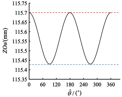
Figure 6. Fluctuation value of point Os on the Zc-axis

图6. Zc轴上Os点的波动值

然后:

V c = V c / / + V c (13b)

其中 V c V c / / 是Vc在动态虚拟相机像素坐标中沿u轴和v轴的分量。

图5所示,基于相似三角形原理, Δ O v c ( t ) O s O v c ( t + T ) Δ L ( t ) O s L ( t + T ) Δ O v c ( t ) O s O v c Δ L ( t ) O s O L ,可以得到:

O v c ( t ) O v c ( t + T ) O s O v c ( t ) = L ( t ) L ( t + T ) O s L ( t ) (14a)

根据公式(6)、公式(9)、公式(13)和公式(14),我们可以计算出动态虚拟相机像素坐标中u轴和v轴的模糊长度:

Δ u = z o s z o v c f z o s z o v c V c T (14b)

Δ v = z o s z o v c f z o s z o v c V c / / T (14c)

然后,像素坐标系中的运动模糊长度Lb,以及运动模糊角度θb可以按如下方式计算:

L b = Δ u 2 + Δ v 2 (14d)

θ b = arctan ( Δ u Δ v ) (14e)

上述表达式表明,运动模糊的长度和方向仅与系统参数、棱镜角度、焦距和动态虚拟相机的光学中心的空间位置Ovc有关。

3.2. 运动模糊消除算法实现

在获得给定图像的运动模糊核的参数后,可以采用维纳滤波法进行运动去模糊处理 [36] 。维纳滤波是一种用于图像去模糊的线性滤波方法,假设扫描图像为 g ( u , v ) ,原始图像为 f ( u , v ) ,运动模糊核为 h ( u , v ) ,以及噪声 n ( u , v ) 。在频域中图像模糊过程可以表示为:

G ( u , v ) = F ( u , v ) H ( u , v ) + N ( u , v ) (15a)

其中, G ( u , v ) F ( u , v ) H ( u , v ) N ( u , v ) 分别是 g ( u , v ) f ( u , v ) h ( u , v ) 和加性噪声 n ( u , v ) 的傅里叶变换。

维纳滤波器的频域表达式为:

W ( u , v ) = H * ( u , v ) / ( | H ( u , v ) | 2 + K ) (15b)

其中, W ( u , v ) 代表维纳滤波器, H * ( u , v ) 是复数共轭, | H ( u , v ) | 2 H ( u , v ) 的平方,K是一个可调参数,用于平衡去模糊化和噪声抑制:

K = | N ( u , v ) | 2 / | F ( u , v ) | 2 (15c)

根据维纳滤波,复原图像 F ( u , v ) 可以用以下表达式计算:

F ( u , v ) = W ( u , v ) * G ( u , v ) (15d)

然后,通过对 F ( u , v ) 进行傅里叶逆变换,得到复原图像 f ( u , v )

f ( u , v ) = I F F T ( F ( u , v ) ) (15e)

基于动态虚拟相机的一阶运动表达式和扫描模糊数学模型,提出了一种实时扫描图像模糊消除算法,如图7所示。

Figure 7. The algorithm of the scanning image deblurring

图7. 扫描图像运动模糊消除算法

4. 实验

实验设备参数如表1所示。

Table 1. The parameter of the prism and camera

表1. 相机棱镜和棱镜的参数

实验中使用的相机焦距为25 mm,相机曝光时间设定为20 ms,通过系统控制器可以获取棱镜1的旋转速度ω1(t),棱镜2的旋转速度ω2(t),以及棱镜的实时旋转位置θ1(t)和θ2(t)。图8(a)和图8(c)是在扫描成像过程中选择的两帧图像。图8(a)所对应的棱镜旋转角度为θ1 = 30˚,θ2 = 30˚,棱镜的旋转速度为ω1 = 30˚/s,ω2 = 30˚/s。图8(c)所对应的棱镜旋转角度为θ1 = 320˚,θ2 = 340˚,棱镜的旋转速度为ω1 = 40˚/s,ω2 = 20˚/s。图8(b)和图8(d)分别是图8(a)和图8(c)的运动模糊消除图像。基于所提出的算法,在配置matlab2020a和i7-9750h@4.0 Ghz处理器的计算机上可以在0.0986 s内完成分辨率为1600 × 1200的图像的运动模糊消除。

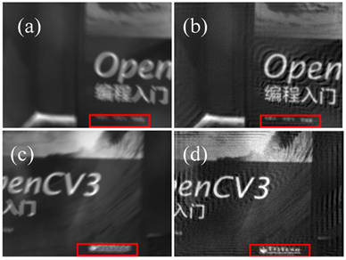
Figure 8. Scanning image motion deblurring. 1st group: (a) The blurred image, (b) is the motion deblurring image of (a); 2nd group: (c) The blurred image, (d) is the motion deblurring image of (c)

图8. 扫描图像运动模糊消除。第1组:(a) 模糊图像,(b) 为(a)的运动模糊消除图像;第2组:(c) 模糊的图像,(d) 为(c)的运动模糊消除图像

运动去模糊方法的效果可以用清晰度评价指标函数来评价,设定模糊图像图8(b)和图8(d)为是清晰图像,其相对清晰度为100%。表2显示了模糊图像的相对清晰度,实验表明,该方法可以有效地提高旋转棱镜–相机成像系统扫描成像的图像清晰度。

Table 2. The relative clarity of blurred image

表2. 模糊图像的相对清晰度

5. 结论

本文提出了一种旋转棱镜–相机成像系统扫描图像的运动模糊核估计方法和运动模糊消除算法。通过建立动态虚拟相机模型,我们提出了一种基于动态虚拟相机的运动模糊核估计方法:该方法基于一阶近似算法对动态虚拟相机进行运动学分析,得到动态虚拟相机的一阶运动表达式,结合旋转棱镜–相机成像系统的参数来建立运动模糊核的数学模型,基于该模型可以获得图像的运动模糊核,最后使用维纳滤波实现了运动模糊消除。实验结果表明,所提出的运动模糊消除算法能有效地消除运动模糊,提高实时扫描成像系统的成像质量。同时本文也验证了一阶近似算法对于旋转棱镜扫描成像分析的有效性,为动态目标跟踪和实时环境扫描提供了有效的解决方案。

基金项目

国家自然科学基金面上项目“动态虚拟相机变视轴立体成像原理与方法”(编号61975152)。

NOTES

*第一作者。

#通讯作者。

参考文献

[1] Xu, Z., Wang, J., Zhao, L., Wang, P. and Fang, J. (2011) An All-Reflective Optical System for the Modulation Transfer Func-tion Measurement of Near-Infrared Focal Plane Arrays. Chinese Journal of Lasers, 38, s116002.
[2] Sandau, R. and Eckardt, A. (1995) The Stereo Camera Family WAOSS/WAAC for Spaceborne/Airborne Applications. XVIII Congress of ISPRS, Vi-enna, 9-14 July 1996, 170-175.
[3] Paparoditis, N., Souchon, J.-P., Martinoty, G. and Pierrot-Deseilligny, M. (2006) High-End Aerial Digital Cameras and Their Impact on the Automation and Quality of the Production Workflow. ISPRS Journal of Photogrammetry and Remote Sensing, 60, 400-412.
https://doi.org/10.1016/j.isprsjprs.2006.06.003
[4] Zhou, Y., Chen, Y., Sun, L., et al. (2020) Analysis on Key Issues of Boresight Adjustment in Imaging Tracking Based on Risley Prisms. Optical Engineering, 59, Article ID: 123104.
https://doi.org/10.1117/1.OE.59.12.123104
[5] Wen, P. (2022) Multivaria-ble Decoupling and Nonlinear Correction Method for Image-Based Closed-Loop Tracking of the Risley Prisms System. Mi-cromachines, 13, Article No. 2096.
https://doi.org/10.3390/mi13122096
[6] Li, A., Li, Q., Deng, Z., et al. (2020) Ris-ley-Prism-Based Visual Tracing Method for Robot Guidance. Journal of the Optical Society of America A, 37, 705-713.
https://doi.org/10.1364/JOSAA.381445
[7] Petrie, G. and Walker, A. (2010) Airborne Digital Imaging Technology: A New Overview. The Photogrammetric Record, 22, 203-225.
https://doi.org/10.1111/j.1477-9730.2007.00446.x
[8] Albertz, J., Ebner, H. and Neukum, G. (1996) The HRSC/WAOSS Camera Experiment on the Mars 96 Mission—A Photogrammetric and Cartographic View of the Project. ISPRS Congress, Vienna, 9-19 July 1996, 476-480.
[9] Lan, Y., Thomson, S., Huang, Y., Hoffmann, W. and Zhang, H. (2010) Current Status and Future Directions of Precision Aerial Application for Site-Specific Crop Management in the USA. Computers & Electronics in Agriculture, 74, 34-38.
https://doi.org/10.1016/j.compag.2010.07.001
[10] Bostater, C., Jones, J., Frystacky, H., Coppin, G. and Neyt, X. (2011) Airborne Imaging Sensors for Environmental Monitoring and Surveillance in Support of Oil Spills and Recovery Efforts. Proceedings SPIE, Remote Sensing of the Ocean, Sea Ice, Coastal Waters, and Large Water Regions, Vol. 8175, 81750B.
https://doi.org/10.1117/12.901231
[11] Rosell, F. (1960) Prism Scanner. Journal of the Optical Society of America, 50, 521-526.
https://doi.org/10.1364/JOSA.50.000521
[12] Li, A., Sun, W., Yi, W. and Zuo, Q. (2016) Investigation of Beam Steering Performances in Rotation Risley-Prism Scanner. Optics Express, 24, 12840-12850.
https://doi.org/10.1364/OE.24.012840
[13] Artamonov, S.I., Gryaznov, N.A., Kuprenyuk, V.I., Romanov, N.A. and Sosnov, E.N. (2016) Selection of Scanners for Use in Lidar Systems. Journal of Optical Technology, 83, 549-555.
https://doi.org/10.1364/JOT.83.000549
[14] Wang, Z., Cao, J., Hao, Q., et al. (2019) Super-Resolution Imaging and Field of View Extension Using a Single Camera with Risley Prisms. The Review of Scientific Instruments, 90, Article ID: 033701.
https://doi.org/10.1063/1.5050833
[15] Chen, Y., Wang, B., Li, Q., et al. (2022) Field-of-View-Enlarged Single-Camera 3D Shape Reconstruction. IEEE Transactions on Instrumentation and Measurement, 71, 1-12.
https://doi.org/10.1109/TIM.2022.3165271
[16] Han, Z. and Zhang, L. (2023) A Virtual Multi-Ocular 3D Reconstruction System Using a Galvanometer Scanner and a Camera. Sensors, 23, Article No. 3499.
https://doi.org/10.3390/s23073499
[17] Zhang, H., Cao, J., Zhou, D., Cui, H., et al. (2022) Three-Dimensional Computa-tional Ghost Imaging Using a Dynamic Virtual Projection Unit Generated by Risley Prisms. Optics Express, 30, 39152-39161.
https://doi.org/10.1364/OE.472889
[18] Church, P., Matheson, J., Cao, X. and Roy, G. (2017) Evaluation of a Steerable 3D Laser Scanner Using a Double Risley Prism Pair. Proceedings of the SPIE Degraded Environments: Sensing, Processing, and Display, Volume 10197, 101970O.
https://doi.org/10.1117/12.2262198
[19] Vuthea, V. and Toshiyoshi, H. (2018) A Design of Risley Scanner for LiDAR Applications. 2018 International Conference on Optical MEMS and Nanophotonics (OMN), Lausanne, 29 July-2 August 2018, 1-2.
https://doi.org/10.1109/OMN.2018.8454641
[20] Lavigne, V. and Ricard, B. (2005) Step-Stare Image Gathering for High-Resolution Targeting. In: Advanced Sensory Payloads for UAV, RTO, Neuilly-sur-Seine, Paper 17.
[21] Li, A., Liu, X., Gong, W., Sun, W. and Sun, J. (2019) Prelocation Image Stitching Method Based on Flexible and Precise Boresight Adjustment Using Risley Prisms. JOSA A, 36, 305-311.
https://doi.org/10.1364/JOSAA.36.000305
[22] Hao, Q., Wang, Z., Cao, J. and Zhang, F. (2018) A Hybrid Bionic Image Sensor Achieving FOV Extension and Foveated Imaging. Sensors, 18, Article No. 1042.
https://doi.org/10.3390/s18041042
[23] Li, A. and Zhong, S. (2019) Calibration Method of Risley-Prism Imaging System. Optics Communications, 459, Article ID: 124975.
https://doi.org/10.1016/j.optcom.2019.124975
[24] Li, A., Liu, X. and Zhao, Z. (2020) Compact Three-Dimensional Computational Imaging Using Dynamic Virtual Camera. Optics Letters, 45, 3801-3804.
https://doi.org/10.1364/OL.395983
[25] Marshall, G.F. (1999) Risley Prism Scan Patterns. Proceedings of the SPIE, 3787, 74-86.
[26] Jeon, Y.-G. (2011) Generalization of the First-Order Formula for Analysis of Scan Patterns of Risley Prisms. Optical Engineering, 50, Article ID: 113002.
https://doi.org/10.1117/1.3655501
[27] Schwarze, C., Vaillancourt, R., Carlson, D., Schundler, E., Evans, T. and Engel, J.R. (2005) Risley-Prism Based Compact Laser Beam Steering for IRCM, Laser Communications, and Laser Radar. Optra Inc., Topsfield.
[28] Lavigne, V. and Ricard, B. (2007) Fast Risley Prisms Camera Steering System: Calibration and Image Distortions Correction through the Use of a Three-Dimensional Refractive Model. Optical Engineering, 46, Article ID: 043201.
https://doi.org/10.1117/1.2722754
[29] Huang, F., Ren, H., Shen, Y. and Wang, P. (2021) Error Analysis and Optimiza-tion for Risley-Prism Imaging Distortion Correction. Applied Optics, 60, 2574-2582.
https://doi.org/10.1364/AO.418007
[30] Dainty, J.C. (1984) Theory and Practice of Scanning Optical Microscopy. Optica Acta: International Journal of Optics, 32, 1451-1452.
https://doi.org/10.1080/713821694
[31] Nemes, M.S., Jr., C.B. and Savoy, H. (2009) A Forward Motion Compensation System for Airborne Remote Sensing Platforms & Aerial Mapping Cam-eras. European Journal of Mechanical and Environmental Engineering, No. 2, 24-28.
[32] Chen, S., Wang, G., Li, X., Zhang, Q., Shi, Z. and Guan, Y. (2020) Formalization of Camera Pose Estimation Algorithm Based on Rodrigues Formula. Formal Aspects of Computing, 32, 417-437.
https://doi.org/10.1007/s00165-020-00520-5
[33] Boisset, G.C., Robertson, B. and Hinton, H.S. (2002) Design and Con-struction of an Active Alignment Demonstrator for a Free-Space Optical Interconnect. IEEE Photonics Technology Letters, 7, 676-678.
https://doi.org/10.1109/68.388762
[34] Moghaddam, M.E. and Jamzad, M. (2007) Motion Blur Identification in Noisy Images Using Mathematical Models and Statistical Measures. Pattern Recognition, 40, 1946-1957.
https://doi.org/10.1016/j.patcog.2006.11.022
[35] Al-Amri, S.S. and Kalyankar, N.V. (2010) A Comparative Study for Deblurred Average Blurred Images. International Journal on Computer Science and Engineering, 2, 731-733.
[36] Gonzalez, R.C. and Woods, R.E. (2010) Digital Image Processing. 3rd Edition, Pearson Education, London, 374-376.