带有几何源项的浅水波方程组的高精度熵稳定有限差分格式

A High Order Entropy Stable Finite Difference Scheme for Shallow Water Equations with Geometric Source Term

摘要: 本文建立了浅水波方程组的有限差分格式，该格式具有高阶精度和保持熵稳定性。首先，我们构造了一个二阶熵守恒格式，该格式满足给定熵对的熵等式，并能准确地保持湖泊静止稳态。主要思想是使源项的离散化与通量梯度项的离散化相匹配。其次，以具有合理熵守恒通量的二阶熵守恒格式为基础，实现了高阶熵守恒格式。第三，在已有的熵守恒格式上增加适当的耗散项，得到满足离散熵不等式的半离散熵稳定格式。特别是熵稳定格式可以避免熵守恒格式的振荡。其中，耗散项的建立采用根据熵变量构造的加权本质无振荡重构。最后，采用龙格–库塔方法进行时间离散化。文中给出了大量的数值算例，以验证该方法的高精度性及解决捕捉间断的能力。

Abstract: In this article, a finite difference scheme for shallow water wave equations with geometric source terms is established, which has high order accuracy and maintains entropy stability. First, we con-struct a second order entropy conservation scheme that satisfies the entropy conservation equation for a given entropy pair and can accurately maintain the stationary state of the lake. The main idea is to match the discretization of the source term with the discretization of the flux gradient term. Secondly, based on the second order entropy conservation scheme with reasonable entropy con-servation flux, a higher order entropy conservation scheme is implemented. Thirdly, by adding ap-propriate dissipation terms to existing entropy conservation schemes, a semi discrete entropy sta-ble scheme satisfying discrete entropy inequality is obtained. In particular, the entropy stable scheme can avoid the oscillation of the entropy conservation scheme. The dissipation term is estab-lished using weighted essentially non oscillatory reconstruction constructed from entropy variables. Finally, the Runge-Kutta method is used for time discretization. A large number of numerical exam-ples are given to verify the high accuracy of the method and its ability to solve capture discontinui-ties.

1. 引言

浅水方程(SWEs)被广泛应用于模拟浅水流体(如河流、海岸流、湖泊流、潮汐等)。其一维(1-D)形式为

$\frac{\partial U}{\partial t}+\frac{\partial F\left(U\right)}{\partial x}=-S\left(U,b\right),$ (1)

其中 $U={\left(h,hu\right)}^{\text{T}},F\left(U\right)={\left(hu,h{u}^2+\frac{1}{2}g{h}^2\right)}^{\text{T}},S\left(U,b\right)={\left(0,gh{b}_x\right)}^{\text{T}}$ ， $h\left(x,t\right)$ 和 $u\left(x,t\right)$ 分别为流体的高度和深度平均速度。这里， $b\left(x\right)$ 表示底部地形， $g=9.812$ 为重力常数。其中， $S\left(U,b\right)={\left(0,gh{b}_x\right)}^{\text{T}}$ 表示由于水体底部不平所造成的几何源项。

特别是方程组(1)保持了以下湖泊静止稳态

$u=0,h+b=\mathrm{Constant}.$ (2)

实际上，由于方程组(1)的高度非线性，对其进行理论分析非常困难。因此，高阶格式数值求解是求解这些问题的有效方法，在计算流体力学领域引起了广泛关注 [1] [2] [3] 。之后出现了很多研究(1)的高阶格式，其中具有代表性的SWEs格式主要有：中心迎风格式 [4] 、加权本质非振荡(WENO)格式 [5] - [14] 、中心格式 [15] [16] [17] [18] 、龙格库塔间断伽辽金(RKDG)方法 [19] [20] [21] 、ADER (时空任意导数)格式 [22] [23] 、Godunov型方法 [24] [25] 、DG谱元方法 [26] 、中心逆风格式 [27] [28] 、ADER-DG方法 [29] 。中心迎风格式是扩展半离散的中信格式且注意源项的离散化；经过多人研究的WENO格式能够保持其原始的高阶精度和一般解的基本非振荡特性；RKDG方法完全保留了等温流体静力状态的W-B特征，用大量示例展示了W-B功能、高阶精度和良好的分辨率；ADER格式具有源项的双曲系统在空间和时间上的高精度，实现并测试了在空间和时间上精度高达五阶的方案。

本文是基于方程组(1)的精确解可能不存在的原因而从分布意义上寻找弱解，但弱解可能不是唯一的。因此，添加一个熵条件来确定一个物理相关的解。事实上，熵条件在所有可能的弱解中筛选熵解起着重要作用。

定义1 (熵函数 [30] )凸函数 $\eta \left(U\right)$ 被称为方程组(1)的熵函数，如果存在满足等式的熵通量 $q\left(U\right)$ 使得

$q^{\prime }\left(U\right)=V^{T}F\left(U\right),$ (3)

其中 $V={\eta }^{\prime }{\left(U\right)}^T$ 为熵变量。相应地，我们称 $\left(\eta ,q\right)$ 为熵对。

对于给定的熵对 $\left(\eta ,q\right)$ ，将(1)的两端乘以 $V^T$ ，(1)的光滑解满足下面的熵等式

$\frac{\partial \eta \left(U\right)}{\partial t}+\frac{\partial q\left(U\right)}{\partial x}=-V^{T}S\left(U,b\right).$ (4)

然而，上述等式(4)在出现间断解的情况下不再成立。特别地，方程组(1)的弱解 $U$ 被称为熵解 [30] ，如果存在熵不等式

$\frac{\partial \eta \left(U\right)}{\partial t}+\frac{\partial q\left(U\right)}{\partial x}\le -V^{T}S\left(U,b\right)，$ (5)

对于给定的熵对 $(\eta ,q)$ 在分布的框架下是成立的。

通常，熵等式(4)和熵不等式(5)都被称为熵条件，这在理论上对(1)等双曲平衡律的适定性起着重要作用。根据(5)满足离散熵不等式的格式也被称为熵稳定(ES)格式。近年来，对于SWEs，具有高鲁棒性的ES格式得到了广泛关注，如DG谱元方法 [31] 、节点DG方法 [32] 、RKDG方法 [33] [34] 、有限差分(FD)格式 [35] [36] 。

本文的主要目的是为中小企业开发一个高阶ES FD格式。首先，我们提出了一种二阶熵守恒(EC)格式，该格式满足熵等式，采用适当的底部地形离散化和两点EC通量。然后，以获得的二阶EC格式为构成元素，得到相应的高阶EC格式。此外，该格式完全保持了湖泊静止稳态，具有well-balanced性质(WB)。

但是，EC格式可能在间断附近引起伪振荡。为了克服这一缺点，我们根据熵变量利用WENO重构构造了合适的耗散项，并将其添加到EC通量中，实现了高阶ES格式。所提出的ES格式满足半离散形式的熵不等式。最后，采用龙格–库塔方法对半离散ES格式进行时间迭代。

本文的内容组织如下：在第二节中，我们提出了一种适用于一维SWEs的EC FD格式。随后，我们在第3节中对提出的格式进行了W-B分析。在第4节中，我们实验了几个经典的例子来证明当前格式的性质。最后，我们在第5节中得出了一些结论。

2. 一维EC格式的构造

为方便起见，方程组(1)有如下等价形式

$\frac{\partial U}{\partial t}+\frac{\partial F\left(U\right)}{\partial x}=-G\frac{\partial b}{\partial x},$ (6)

其中 $G={\left(0,gh\right)}^T.$ 其中，对于一维SWEs(6)，我们取总能量

$\eta =\eta \left(U\right)=\frac{1}{2}\left(h{u}^2+g{h}^2\right)+ghb,$

作为数学熵函数 [30] [36] 与

$V=\eta \text{'}{\left(U\right)}^T={\left(g\left(h+b\right)-\frac{1}{2}{u}^2,u\right)}^T$

作为熵变量。相应地，根据(3)的一致条件熵通量为

$q=q\left(U\right)=\frac{1}{2}h{u}^3+g{h}^{2}u+ghub.$

此外，我们假定

$\psi =V^{T}F\left(U\right)-q\left(U\right)=\frac{1}{2}g{h}^{2}u$

作为熵势。

首先，我们将空间域划分为以 $x_0<x_1<\cdots <x_N$ 为网格节点的均匀网格，并以 $\Delta x=x_i-x_{i-1}$ 为空间步长。(6)的FD格式为

$\frac{\text{d}}{\text{d}t}{U}_i=-\frac{1}{\Delta x}\left({\tilde{F}}_{i+\frac{1}{2}}-{\tilde{F}}_{i-\frac{1}{2}}\right)-G_i\frac{{\left\{\left\{b\right\}\right\}}_{i+\frac{1}{2}}-{\left\{\left\{b\right\}\right\}}_{i-\frac{1}{2}}}{\Delta x},$ (7)

其中，符号 ${\left\{\left\{a\right\}\right\}}_{i+\frac{1}{2}}=\frac{1}{2}\left(a_i+a_{i+1}\right)$ 表示 $a$ 在点 $x_{i+\frac{1}{2}}=x_i+\Delta x/2$ 处的平均值。此外，这里使用数值通量 ${\tilde{F}}_{i+\frac{1}{2}}$ 来近似 $x_{i+\frac{1}{2}}$处的物理通量 $F\left(U\right)$ 。然后，我们着重构造数值通量 ${\tilde{F}}_{i+\frac{1}{2}}$ 。

特别地，式(7)的解满足以下半离散熵等式

$\frac{\text{d}}{\text{d}t}\eta \left(U_i\right)+\frac{1}{\Delta x}\left({\tilde{q}}_{i+\frac{1}{2}}-{\tilde{q}}_{i-\frac{1}{2}}\right)=0,$ (8)

那么格式(7)被称为EC格式。这里需要数值熵通量 ${\tilde{q}}_{i+\frac{1}{2}}$ 与给定熵通量q保持一致，则数值熵通量 ${\tilde{F}}_{i+\frac{1}{2}}$ 即为EC通量。实际上，式(8)根据等式(4)表示离散状态。

下面引理给出了格式(7)为EC的充分条件，以及源项离散化。

引理1 给定格式(7)称为EC，是二阶格式，条件是数值通量 ${\tilde{F}}_{i+\frac{1}{2}}：=F\left(U_i,U_{i+1}\right)$ 在(7)中满足

${\left[\left[V\right]\right]}^T\tilde{F}=\left[\left[\psi \right]\right]+g\left[\left[hub\right]\right]-g\left[\left[hu\right]\right]\left\{\left\{b\right\}\right\},$ (9)

其中 $\left\{\left\{a\right\}\right\}=\frac{1}{2}\left(a_i+a_{i+1}\right),\left[\left[a\right]\right]=a_{i+1}-a_i$ 。(8)中的数值熵通量 ${\tilde{q}}_{i+\frac{1}{2}}$ 为

${\tilde{q}}_{i+\frac{1}{2}}={\left\{\left\{V\right\}\right\}}_{i+\frac{1}{2}}^T{\tilde{F}}_{i+\frac{1}{2}}-{\left\{\left\{\psi \right\}\right\}}_{i+\frac{1}{2}}+g{\left\{\left\{hu\right\}\right\}}_{i+\frac{1}{2}}{\left\{\left\{b\right\}\right\}}_{i+\frac{1}{2}}-g{\left\{\left\{hub\right\}\right\}}_{i+\frac{1}{2}}.$ (10)

证明 (7)两端左乘 $V_i^T$ 得到

$\frac{\text{d}{\eta }_i}{\text{d}t}=-\frac{1}{\Delta x}\left[V_i^T\left({\tilde{F}}_{i+\frac{1}{2}}-{\tilde{F}}_{i-\frac{1}{2}}\right)+g{h}_i{u}_i\left({\left\{\left\{b\right\}\right\}}_{i+\frac{1}{2}}-{\left\{\left\{b\right\}\right\}}_{i-\frac{1}{2}}\right)\right].$

然后有

$\begin{array}{l}{V}_i^T\left({\tilde{F}}_{i+\frac{1}{2}}-{\tilde{F}}_{i-\frac{1}{2}}\right)+g{h}_i{u}_i\left({\left\{\left\{b\right\}\right\}}_{i+\frac{1}{2}}-{\left\{\left\{b\right\}\right\}}_{i-\frac{1}{2}}\right)\\ ={\left({\left\{\left\{V\right\}\right\}}_{i+\frac{1}{2}}-\frac{1}{2}{\left[\left[V\right]\right]}_{i+\frac{1}{2}}\right)}^T{\tilde{F}}_{i+\frac{1}{2}}-{\left({\left\{\left\{V\right\}\right\}}_{i-\frac{1}{2}}+\frac{1}{2}{\left[\left[V\right]\right]}_{i-\frac{1}{2}}\right)}^T{\tilde{F}}_{i-\frac{1}{2}}\\ +g\left({\left\{\left\{hu\right\}\right\}}_{i+\frac{1}{2}}-\frac{1}{2}{\left[\left[hu\right]\right]}_{i+\frac{1}{2}}\right){\left\{\left\{b\right\}\right\}}_{i+\frac{1}{2}}-g\left({\left\{\left\{hu\right\}\right\}}_{i-\frac{1}{2}}+\frac{1}{2}{\left[\left[hu\right]\right]}_{i-\frac{1}{2}}\right){\left\{\left\{b\right\}\right\}}_{i-\frac{1}{2}}\\ ={\left\{\left\{V\right\}\right\}}_{i+\frac{1}{2}}^T{\tilde{F}}_{i+\frac{1}{2}}-\frac{1}{2}{\left[\left[\psi \right]\right]}_{i+\frac{1}{2}}-\frac{1}{2}g{\left[\left[hbu\right]\right]}_{i+\frac{1}{2}}+\frac{1}{2}g{\left[\left[hu\right]\right]}_{i+\frac{1}{2}}{\left\{\left\{b\right\}\right\}}_{i+\frac{1}{2}}\\ +g{\left\{\left\{hu\right\}\right\}}_{i+\frac{1}{2}}{\left\{\left\{b\right\}\right\}}_{i+\frac{1}{2}}-\frac{1}{2}g{\left[\left[hu\right]\right]}_{i+\frac{1}{2}}{\left\{\left\{b\right\}\right\}}_{i+\frac{1}{2}}\end{array}$

$\begin{array}{l}-{\left\{\left\{V\right\}\right\}}_{i-\frac{1}{2}}^T{\tilde{F}}_{i-\frac{1}{2}}-\frac{1}{2}{\left[\left[\psi \right]\right]}_{i-\frac{1}{2}}-\frac{1}{2}g{\left[\left[hbu\right]\right]}_{i-\frac{1}{2}}+\frac{1}{2}g{\left[\left[hu\right]\right]}_{i-\frac{1}{2}}{\left\{\left\{b\right\}\right\}}_{i-\frac{1}{2}}\\ -g{\left\{\left\{hu\right\}\right\}}_{i-\frac{1}{2}}{\left\{\left\{b\right\}\right\}}_{i-\frac{1}{2}}-\frac{1}{2}g{\left[\left[hu\right]\right]}_{i-\frac{1}{2}}{\left\{\left\{b\right\}\right\}}_{i-\frac{1}{2}}\\ =\left({\left\{\left\{V\right\}\right\}}_{i+\frac{1}{2}}^T{\tilde{F}}_{i+\frac{1}{2}}-{\left\{\left\{\psi \right\}\right\}}_{i+\frac{1}{2}}+g{\left\{\left\{hu\right\}\right\}}_{i+\frac{1}{2}}{\left\{\left\{b\right\}\right\}}_{i+\frac{1}{2}}-g{\left\{\left\{hbu\right\}\right\}}_{i+\frac{1}{2}}\right)\\ -\left({\left\{\left\{V\right\}\right\}}_{i-\frac{1}{2}}^T{\tilde{F}}_{i-\frac{1}{2}}-{\left\{\left\{\psi \right\}\right\}}_{i-\frac{1}{2}}+g{\left\{\left\{hu\right\}\right\}}_{i-\frac{1}{2}}{\left\{\left\{b\right\}\right\}}_{i-\frac{1}{2}}-g{\left\{\left\{hbu\right\}\right\}}_{i-\frac{1}{2}}\right)\\ :={\tilde{q}}_{i+\frac{1}{2}}-{\tilde{q}}_{i-\frac{1}{2}}.\end{array}$

这里 $a_i={\left\{\left\{a\right\}\right\}}_{i+\frac{1}{2}}-\frac{1}{2}{\left[\left[a\right]\right]}_{i+\frac{1}{2}}$ 和 $a_i={\left\{\left\{a\right\}\right\}}_{i-\frac{1}{2}}+\frac{1}{2}{\left[\left[a\right]\right]}_{i-\frac{1}{2}}$ 已应用于上述第一个方程；充分条件(9)以及等式 $\frac{1}{2}{\left[\left[a\right]\right]}_{i+\frac{1}{2}}+\frac{1}{2}{\left[\left[a\right]\right]}_{i-\frac{1}{2}}={\left\{\left\{a\right\}\right\}}_{i+\frac{1}{2}}-{\left\{\left\{a\right\}\right\}}_{i-\frac{1}{2}}$ 已用于第二个和第三个。因此，格式(7)用 ${\tilde{F}}_{i+\frac{1}{2}}={\tilde{F}}_{i+\frac{1}{2}}\left(U_i,U_{i+1}\right)$ 对(8)进行EC模拟。

此外，(7)中的源项离散化采用了二阶中心差分。此外，从 [37] 开始对通量梯度的离散也是二阶精确的。因此，格式(7)最终具有二阶精度。

接下来，我们给出了满足充分条件(9)的EC通量。

定理2 对于1-d SWES (1)，数值通量

$\tilde{F}=\left(\begin{array}{c}\left\{\left\{h\right\}\right\}\left\{\left\{u\right\}\right\}\\ \left\{\left\{h\right\}\right\}{\left\{\left\{u\right\}\right\}}^2+\frac{g}{2}\left\{\left\{h^2\right\}\right\}+g\left(\left\{\left\{hb\right\}\right\}-\left\{\left\{h\right\}\right\}\left\{\left\{b\right\}\right\}\right)\end{array}\right)$ (11)

为EC通量，与(1)中的物理通量 $F\left(U\right)$ 兼容。

证明 在这里，重点在于我们使用下面的恒等式

$\left[\left[ab\right]\right]=\left\{\left\{a\right\}\right\}\left[\left[b\right]\right]+\left[\left[a\right]\right]\left\{\left\{b\right\}\right\},$

并应用下面跳跃的等价形式

${\left[\left[V\right]\right]}^T={\left(g\left[\left[h\right]\right]+g\left[\left[b\right]\right]-\left\{\left\{u\right\}\right\}\left[\left[u\right]\right],\left[\left[u\right]\right]\right)}^T,$

$\left[\left[\psi \right]\right]=g\left\{\left\{h\right\}\right\}\left\{\left\{u\right\}\right\}\left[\left[h\right]\right]+\frac{1}{2}g\left\{\left\{h^2\right\}\right\}\left[\left[u\right]\right],$

$g\left[\left[hub\right]\right]-g\left[\left[hu\right]\right]\left\{\left\{b\right\}\right\}=g\left\{\left\{h\right\}\right\}\left\{\left\{u\right\}\right\}\left[\left[b\right]\right]+g\left\{\left\{hb\right\}\right\}\left[\left[u\right]\right]-g\left\{\left\{h\right\}\right\}\left\{\left\{b\right\}\right\}\left[\left[u\right]\right].$

然后将上述表达式代入(9)，得到

$\begin{array}{c}\left(g\left[\left[h\right]\right]+g\left[\left[b\right]\right]-\left\{\left\{u\right\}\right\}\left[\left[u\right]\right]\right)\cdot {\tilde{F}}^1+\left[\left[u\right]\right]\cdot {\tilde{F}}^2\\ =g\left\{\left\{h\right\}\right\}\left\{\left\{u\right\}\right\}\left[\left[h\right]\right]+\frac{1}{2}g\left\{\left\{h^2\right\}\right\}\left[\left[u\right]\right]+\left\{\left\{h\right\}\right\}\left\{\left\{u\right\}\right\}\left\{\left\{u\right\}\right\}\left[\left[u\right]\right]-\left\{\left\{h\right\}\right\}\left\{\left\{u\right\}\right\}\left\{\left\{u\right\}\right\}\left[\left[u\right]\right]\\ +g\left\{\left\{h\right\}\right\}\left\{\left\{u\right\}\right\}\left[\left[h\right]\right]+g\left\{\left\{hb\right\}\right\}\left[\left[u\right]\right]-g\left\{\left\{h\right\}\right\}\left\{\left\{b\right\}\right\}\left[\left[u\right]\right]\\ =\left(g\left[\left[h\right]\right]+g\left[\left[b\right]\right]-\left\{\left\{u\right\}\right\}\left[\left[u\right]\right]\right)\cdot \left\{\left\{h\right\}\right\}\left\{\left\{u\right\}\right\}\\ +\left[\left[u\right]\right]\cdot \left(\left\{\left\{h\right\}\right\}{\left\{\left\{u\right\}\right\}}^2+\frac{1}{2}g\left\{\left\{h^2\right\}\right\}+g\left(\left\{\left\{hb\right\}\right\}-\left\{\left\{h\right\}\right\}\left\{\left\{b\right\}\right\}\right)\right).\end{array}$

然后，我们得到下面的恒等式

$\begin{array}{l}\left(g\left[\left[h\right]\right]+g\left[\left[b\right]\right]-\left\{\left\{u\right\}\right\}\left[\left[u\right]\right]\right)\cdot {\tilde{F}}^1=\left(g\left[\left[h\right]\right]+g\left[\left[b\right]\right]-\left\{\left\{u\right\}\right\}\left[\left[u\right]\right]\right)\cdot \left\{\left\{h\right\}\right\}\left\{\left\{u\right\}\right\},\\ \left[\left[u\right]\right]\cdot {\tilde{F}}^2=\left[\left[u\right]\right]\cdot \left(\left\{\left\{h\right\}\right\}{\left\{\left\{u\right\}\right\}}^2+\frac{1}{2}g\left\{\left\{h^2\right\}\right\}+g\left(\left\{\left\{hb\right\}\right\}-\left\{\left\{h\right\}\right\}\left\{\left\{b\right\}\right\}\right)\right)\end{array}$

通过比较同一跳系数，得到

$\begin{array}{l}{\tilde{F}}^1=\left\{\left\{h\right\}\right\}\left\{\left\{u\right\}\right\},\\ {\tilde{F}}^2=\left\{\left\{h\right\}\right\}{\left\{\left\{u\right\}\right\}}^2+\frac{1}{2}g\left\{\left\{h^2\right\}\right\}+g\left(\left\{\left\{hb\right\}\right\}-\left\{\left\{h\right\}\right\}\left\{\left\{b\right\}\right\}\right).\end{array}$

因此，我们最终得到(11)中的数值通量 $\tilde{F}$ 。

备注1 此外，令 $\left(h_L,u_L,b_L\right)=\left(h_R,u_R,b_R\right)=\left(h,u,b\right)$ 在(11)中可得

${\tilde{F}}^1=hu,{\tilde{F}}^2=h{u}^2+\frac{1}{2}g{h}^2.$

因此，(11)中的EC通量 $\tilde{F}$ 与物理通量 $F\left(U\right)$ 是相一致的。

3. W-B性质分析

在这里，我们总结下该格式的W-B性质，并提出下面的定理。

定理3. EC通量为(11)的格式(7)为W-B，并保持湖静止稳态(2)，即(7)的解满足

$\frac{\text{d}}{\text{d}t}{h}_i\equiv 0$ 和 $\frac{\text{d}}{\text{d}t}{\left(hu\right)}_i\equiv 0,$

其中 $u_i\equiv 0,h_i+b_i\equiv \text{Constant},\forall i$ 。

证明 首先，在 $u_i\equiv 0,h_i+b_i\equiv \text{Constant}$ 的假设下，由(11)可知 ${\tilde{F}}^1=0$ ，由(7)可知 $\frac{\text{d}}{\text{d}t}{h}_i\equiv 0$ 。

其次，我们有

$\begin{array}{l}\frac{\text{d}}{\text{d}t}{\left(hu\right)}_i=-\frac{1}{\Delta x}\left({\tilde{F}}_{i+\frac{1}{2}}^2-{\tilde{F}}_{i-\frac{1}{2}}^2\right)-G_i\frac{{\left\{\left\{b\right\}\right\}}_{i+\frac{1}{2}}-{\left\{\left\{b\right\}\right\}}_{i-\frac{1}{2}}}{\Delta x},\\ =-\frac{g}{\Delta x}[\left(\frac{1}{2}{\left\{\left\{h^2\right\}\right\}}_{i+\frac{1}{2}}-\frac{1}{2}{\left\{\left\{h^2\right\}\right\}}_{i-\frac{1}{2}}\right)+\left({\left\{\left\{hb\right\}\right\}}_{i+\frac{1}{2}}-{\left\{\left\{hb\right\}\right\}}_{i-\frac{1}{2}}\right)\\ -\left({\left\{\left\{h\right\}\right\}}_{i+\frac{1}{2}}{\left\{\left\{b\right\}\right\}}_{i+\frac{1}{2}}-{\left\{\left\{h\right\}\right\}}_{i-\frac{1}{2}}{\left\{\left\{b\right\}\right\}}_{i-\frac{1}{2}}\right)+h_i\left({\left\{\left\{b\right\}\right\}}_{i+\frac{1}{2}}-{\left\{\left\{b\right\}\right\}}_{i-\frac{1}{2}}\right)]\\ =-\frac{g}{\Delta x}[\left(\frac{1}{2}{\left\{\left\{h\right\}\right\}}_{i+\frac{1}{2}}{\left[\left[h\right]\right]}_{i+\frac{1}{2}}+\frac{1}{2}{\left\{\left\{h\right\}\right\}}_{i-\frac{1}{2}}{\left[\left[h\right]\right]}_{i-\frac{1}{2}}\right)+\left({\left\{\left\{h\right\}\right\}}_{i+\frac{1}{2}}{b}_{i+1}-{\left\{\left\{h\right\}\right\}}_{i-\frac{1}{2}}{b}_{i-1}\right)\\ -\left({\left\{\left\{h\right\}\right\}}_{i+\frac{1}{2}}{\left\{\left\{b\right\}\right\}}_{i+\frac{1}{2}}-{\left\{\left\{h\right\}\right\}}_{i-\frac{1}{2}}{\left\{\left\{b\right\}\right\}}_{i-\frac{1}{2}}\right)]\end{array}$ (12)

$\begin{array}{l}=-\frac{g}{\Delta x}\left[\left(\frac{1}{2}{\left\{\left\{h\right\}\right\}}_{i+\frac{1}{2}}{\left[\left[h\right]\right]}_{i+\frac{1}{2}}+\frac{1}{2}{\left\{\left\{h\right\}\right\}}_{i-\frac{1}{2}}{\left[\left[h\right]\right]}_{i-\frac{1}{2}}\right)+\frac{1}{2}\left({\left\{\left\{h\right\}\right\}}_{i+\frac{1}{2}}{\left[\left[b\right]\right]}_{i+\frac{1}{2}}+{\left\{\left\{h\right\}\right\}}_{i-\frac{1}{2}}{\left[\left[h\right]\right]}_{i-\frac{1}{2}}\right)\right]\\ =-\frac{g}{2\Delta x}\left[\left({\left\{\left\{h\right\}\right\}}_{i+\frac{1}{2}}{\left[\left[h+b\right]\right]}_{i+\frac{1}{2}}+{\left\{\left\{h\right\}\right\}}_{i-\frac{1}{2}}{\left[\left[h+b\right]\right]}_{i-\frac{1}{2}}\right)\right]\\ \equiv 0,\end{array}$

其中等式 $\frac{1}{2}{\left\{\left\{h^2\right\}\right\}}_{i+\frac{1}{2}}-\frac{1}{2}{\left\{\left\{h^2\right\}\right\}}_{i-\frac{1}{2}}=\frac{1}{2}{\left\{\left\{h\right\}\right\}}_{i+\frac{1}{2}}{\left[\left[h\right]\right]}_{i+\frac{1}{2}}+\frac{1}{2}{\left\{\left\{h\right\}\right\}}_{i-\frac{1}{2}}{\left[\left[h\right]\right]}_{i-\frac{1}{2}}$ 已用于第二个等式。另外， $\left[\left[h+b\right]\right]\equiv 0$ 导致最后一个等式，因为 $h_i+b_i\equiv \text{Constant},\forall i$ 。因此，该格式即为W-B的。

4. 数值结果

在本节中，我们将通过计算不同算例来测试所提出的熵稳定方法的性能。我们在整个计算过程中取重力常数g为9.812，为了保持数值稳定性取 $CFL=0.6$ 。另外，时间离散采用三阶Runge-Kutta方式，

$\begin{array}{l}{U}^{\left(1\right)}=U^n+\Delta tF\left(U^n\right),\\ U^{\left(2\right)}=\frac{3}{4}{U}^n+\frac{1}{4}\left(U^{\left(1\right)}+\Delta tF\left(U^{\left(1\right)}\right)\right),\\ U^{n+1}=\frac{1}{3}{U}^n+\frac{2}{3}\left(U^{\left(2\right)}+\Delta tF\left(U^{\left(2\right)}\right)\right).\end{array}$ (13)

ε = 0.2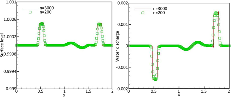ε = 0.001

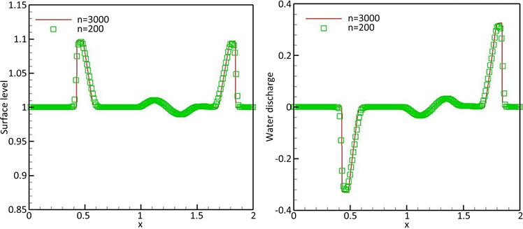
Figure 1. Surface level h + b (left) and water discharge hu (right) at t = 0.2

图1. t = 0.2时的水体表面h + b (左)和出水hu (右)

4.1. 定常水流的扰动问题

这个例子被用来测试该格式捕捉小扰动的能力。初始条件为

$h\left(x,0\right)=\{\begin{array}{l}1-b\left(x\right)+\epsilon \text{if}1.1\le x\le 1.2,\\ 1-b\left(x\right)\text{otherwise,}\end{array}\text{and}u\left(x,0\right)=0,$

水体表面为 $\epsilon >0$ 的凹凸状

$b\left(x\right)=\{\begin{array}{l}0.25\left(\cos \left(10\pi \left(x-1.5\right)\right)+1\right)\text{if}1.4\le x\le 1.6,\\ 0\text{otherwise},\end{array}x\in \left[0,2\right].$

随着时间的推移，初始扰动分解为两个不同方向的脉冲，如图1所示。这两种类型的脉冲都被很好地分辨出来，并且与文献 [7] 中的脉冲很好地吻合。

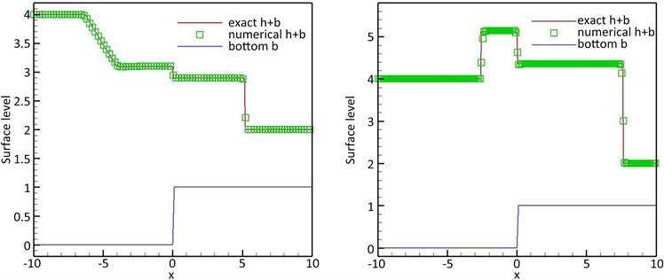
4.2. 一个矩形凸起上的溃坝问题

我们模拟一个溃坝问题 [5] [7] [12] [38] ，并使用以下初始条件

$h\left(x,0\right)=\{\begin{array}{l}20-b\left(x\right)\text{if}x\le 750,\\ 15-b\left(x\right)\text{otherwise,}\end{array}u\left(x,0\right)=0,$

底部为矩形

$b\left(x\right)=\{\begin{array}{l}8\text{if}\left|x-750\right|\le 1500/8,\\ 0\text{otherwise},\end{array}x\in \left[0,1500\right].$

图2分别为t = 15和t = 60时的水体表面。从图2可以看出，该格式得到了较好的结果，与 [5] [7] [12] [38] 中的参考解吻合较好。

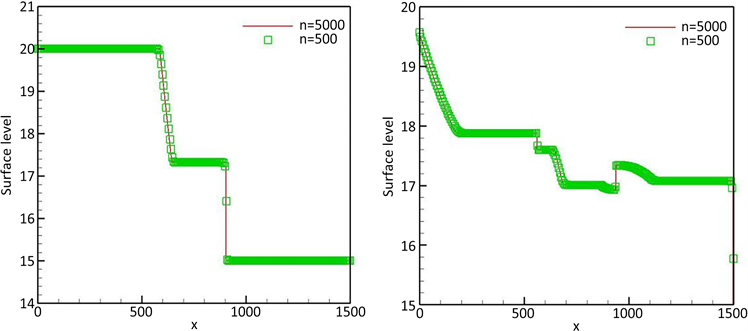
Figure 2. Surface level h + b at t = 15 (left) and t = 60 (right)

图2. t = 15 (左)和t = 60 (右)时的表面h + b

4.3. 过驼峰的一个平稳流

进一步，我们用一个广泛使用的例子 [39] 验证了该格式。实际上，本例基于以下初始数据对跨临界流和次临界流进行了建模

$h\left(x,0\right)=0.33\text{and}u\left(x,0\right)=0,x\in \left[0,25\right]$

底部区域为驼峰

$b\left(x\right)=\{\begin{array}{l}\left(0.2-0.05{\left(x-10\right)}^2\right)\text{if}8\le x\le 12,\\ 0\text{otherwise}.\end{array}$

随后，我们在计算区域的两端实施不同的边界条件。此外，我们还展示了从 [40] 得到的精确解，以提供更好的比较。

• A：无激波的跨临界流动

上游边界的排水量hu = 1.53，下游边界的水深h = 0.66。

• B：带激波的跨临界流

上游边界和下游边界分别施加排水量hu = 0.18和水深h = 0.33。

• C：亚临界流

在上游边界施加流量hu = 4.42，在下游边界施加水深h = 2。

图3给出了上述三种情况的计算结果，表明数值计算结果与实际情况吻合较好。

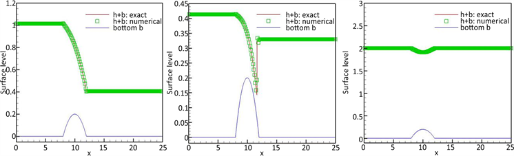A B C

Figure 3. Surface level h + b at t = 200

图3. t = 200时，表面h + b

4.4. Riemann问题

这里，我们用数值方法模拟了一个底部地形为台阶上的断裂例子。

• A

此外，我们使用下面的初始数据实现了一个来自 [41] 的示例

$\left(h,u\right)\left(x,0\right)=\{\begin{array}{l}\left(4,0\right)\text{if}x\le 10,\\ \left(1,0\right)\text{otherwise},\end{array}x\in \left[10,10\right]$

以及一个台阶一样的底部

$b\left(x\right)=\{\begin{array}{l}0\text{if}x\le 0,\\ 1\text{otherwise}.\end{array}$

随着时间的推移，这个例子产生了一个向左移动的稀薄层和一个向右移动的激波。

• B

初始数据为

$\left(h,u\right)\left(x,0\right)=\{\begin{array}{l}\left(4,5\right)\text{if}x\le 10,\\ \left(1,-0.9\right)\text{otherwise},\end{array}x\in \left[10,10\right]$

基于上面同样的底部。随着时间的推移，这个例子出现了两个向不同方向移动的冲击。

• C

本算例来自 [42] ，初始条件为

$\left(h,u\right)\left(x,0\right)=\{\begin{array}{l}\left(0.75,-9.49365\right)\text{if}x\le 0,\\ \left(1.10594,-4.94074\right)\text{otherwise},\end{array}x\in \left[-15,5\right]$

基于以下底部

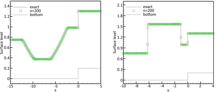A BC D

Figure 4. Surface level h + b at t = 1

图4. t = 1时的表面h + b

$b\left(x\right)=\{\begin{array}{l}0\text{if}x\le 0,\\ 0.2\text{otherwise}.\end{array}$

• D

初始数据为

$\left(h,u\right)\left(x,0\right)=\{\begin{array}{l}\left(0.75,-1.35624\right)\text{if}x\le 0,\\ \left(1.10594,-4.94074\right)\text{otherwise},\end{array}x\in \left[-10,4\right]$

其中，底部地形与情形C一致

图4显示了上述四个例子与精确解的对比结果，清楚地表明了良好的一致性。

5. 结论

本文提出了一种适用于底层地形的一维ES FD格式。首先，我们构造了满足给定熵对的离散熵恒等的二阶EC FD格式，同时保持湖泊静止稳态；关键的思想是同时匹配通量梯度和几何源项。然而，EC格式可能在间断附近产生伪振荡，因此我们在EC通量中加入适当的耗散项。本文采用基于尺度熵变量的WENO重构方法构建耗散项。

最后，我们采用龙格–库塔方式进行时间离散化。此外，大量的实例表明，所提出的格式是W-B，具有较高的精度，并能很好地解决小扰动。

基金项目

本研究的作者钱守国得到了山东省自然科学基金资助项目(ZR2021MA072)的支持。

NOTES

^*通讯作者。