浅水波方程组的熵稳定有限体积格式
Entropy Stable Finite Volume Scheme for Shallow Water Equations
摘要: 本文针对非平底地形上的浅水波方程组,提出了一种高精度熵稳定有限体积格式。首先,我们构造了一个具有二阶精度的well-balanced的半离散熵守恒格式,该格式满足给定熵对的熵恒等式,并精确地保持静水稳态。本文的关键点是使通量梯度和源项的离散化相互匹配;其次,二阶熵守恒格式的可负担熵守恒通量对于最终的高阶格式也是至关重要的。然后,以二阶熵守恒格式为基本模块,实现了高阶well-balanced的半离散熵守恒格式。第三,通过在现有的熵守恒格式中添加适当的耗散项,提出了高阶精度的well-balanced的半离散熵稳定格式,该耗散项基于标度熵变量的加权本质非振荡重构,以克服熵守恒的数值振荡。最后,使用Runge-Kutta方法对半离散格式进行时间积分,以实现最终格式。用大量的数值结果说明所提出的格式满足离散熵不等式,具有良好的平衡性,保持了光滑解的真正高阶精度,并且能够很好地捕获稳态下的小扰动。
Abstract: This article develops a high-order accurate entropy stable finite volume scheme for the shallow wa-ter equations over non-flat bottom topography. Firstly, we construct a second-order accurate well-balanced semi-discrete entropy conservative scheme, which satisfies the entropy identity for the given entropy pair and maintains the still water steady states exactly. The key idea is to make both discretizations for the flux gradient and the source term match each other. Secondly, afforda-ble entropy conservative fluxes of the second-order entropy conservative schemes are also critical for the ultimate high-order scheme. Then, high-order well-balanced semi-discrete entropy con-servative scheme is achieved by taking the second-order entropy conservative schemes as a build-ing block. Thirdly, the high-order accurate well-balanced semi-discrete entropy stable schemes are proposed by adding a suitable dissipation term to the existing entropy conservative scheme based on the weighted essentially non-oscillatory reconstruction of the scaled entropy variables to sup-press the numerical oscillations of the entropy conservative scheme. Finally, the semi-discrete scheme is integrated in time using the Runge-Kutta approach to achieve the eventual scheme. Ex-tensive numerical results strongly indicate that the proposed scheme satisfies the discrete entropy inequality, is well-balanced, keeps the genuine high-order accuracy for smooth solutions, and can well capture small perturbations according to the steady state.
文章引用:刘仁迪, 赵晓旭, 钱守国, 李刚. 浅水波方程组的熵稳定有限体积格式[J]. 应用数学进展, 2023, 12(4): 1908-1926. https://doi.org/10.12677/AAM.2023.124197

1. 引言

浅水波方程组(SWE)广泛用于描述在重力和底部地形影响下的浅水流(如河流和海岸流、湖泊流、潮汐等),其垂直维度远小于水平维度。其一维形式为

U t + F ( U ) x = S ( U , b ) , (1)

其中守恒变量 U = ( h , h u ) T ,物理通量 F ( U ) = ( h u , h u 2 + 1 2 g h 2 ) T ,以及源项 S ( U , b ) = ( 0 , g h b x ) T 。其中,

h ( x , t ) 表示流体的高度, u ( x , t ) 表示流体速度的深度平均, b ( x ) 表示底部地形, g = 9.812 表示重力常数。特别的,方程组(1)满足下面的静水稳态方程

u = 0 , h + b = Constant . (2)

实际上,由于控制方程的高度非线性,方程组(1)的理论分析非常困难。因此,高阶格式的数值求解是解决这些问题的有效方法,并在计算流体力学领域引起了广泛关注 [1] [2] [3] 。SWE高阶格式的代表性研究(1)主要包括:动理学格式 [4] 、气体动理学格式 [5] 、中心迎风格式 [6] 、加权基本非振荡(WENO)格式 [7] - [16] 、Hermite WENO格式 [17] 、中心格式 [18] [19] [20] [21] 、Runge-Kutta间断Galerkin (RKDG)方法 [22] [23] [24] 、ADER (Arbitrary DERivatives in space and time)格式 [25] [26] 、谱元法 [27] 、Godunov方法 [28] [29] 、无网格伽辽金法 [30] 、中心–迎风格式 [31] [32] 、ADER间断伽辽金(ADER-DG)法 [33] 。

此外,非线性双曲守恒律(如方程组(1))一般没有精确解。因此,需要定义弱解。不幸的是,这种弱解可能不是唯一的。事实上,熵条件从所有可能的弱解中筛选物理相关解方面起着重要作用。此外,物理相关解也称为熵解。

定义1. (熵函数 [34] )严格凸函数 η ( U ) 称为方程组(1)的熵函数,如果存在相关的熵通量 q ( U ) ,使得

q ( U ) = V T F ( U ) , (3)

其中 V = η ( U ) T 称为熵变量, ( η , q ) 称为熵对。

对于给定的熵对 ( η , q ) ,将(1)的两端乘以 V T ,其光滑解满足以下熵恒等式

η ( U ) t + q ( U ) x = V T S ( U , b ) , (4)

然而,在出现间断解的情况下,上述恒等式(4)不再成立。特别地,如果对于所有给定的熵对 ( η , q ) ,能使

η ( U ) t + q ( U ) x V T S ( U , b ) , (5)

在分布意义上成立,则(1)的弱解 U 被称为熵解(或物理相关解) [34] 。

通常,熵恒等式(4)和熵不等式(5)都被称为熵条件。理论上,熵条件对于双曲平衡定律(如(1))的适定性非常重要;数值上,满足(5)所述离散熵不等式的高阶格式可以提高其自身的鲁棒性。因此,对于给定的熵对,构造满足离散熵不等式(5)的数值格式具有重要意义。满足离散熵不等式的格式也称为熵稳定格式。近年来,熵稳定格式受到了广泛的关注。浅水波方程组的高阶熵稳定(ES)格式主要包括:间断Galerkin谱元法 [35] ,节点间断Galerkin方法 [36] ,间断Gallerkin (DG)方法 [37] [38] ,有限差分格式 [39] [40] 。

本文的主要目的是提出非平底地形上一维和二维SWE的高阶ES格式。通过对非平底地形进行适当的离散化,提出了两点熵守恒(EC)通量来构造满足熵恒等式的半离散二阶精确平衡EC格式。然后,以上述两点EC格式为构建块,相应地实现了高阶well-balanced的EC格式。然而,EC格式可能会在间断性周围产生数值振荡。为了克服这一缺点,考虑到尺度熵变量,使用WENO重构将一些合适的耗散项添加到EC通量中,以实现满足半离散熵不等式的高阶精确平衡ES格式。半离散EC格式和ES格式都与高阶Runge-Kutta方法相结合,用于时间离散。

本文的组织如下:在第2节中,我们给出了一维SWE的平衡EC有限体积格式。随后,我们在第3节中将所提出的格式扩展到二维领域。在第4节中,我们给出了大量的数值示例,以证明所得格式的性质。最后,第5节得出了相关结论。

2. 一维EC格式的构造

为方便起见,原始控制方程(1)可以改写如下

U t + F ( U ) x = G b x , (6)

其中 G = ( 0 , g h ) T 。这里,对于一维SWE (6),我们将总能量作为数学熵函数 [34] [40]

η = η ( U ) = 1 2 ( h u 2 + g h 2 ) + g h b ,

以及由下式给出的熵变量

V = η ( U ) T = ( g ( h + b ) 1 2 u 2 , u ) T .

因此,考虑到一致条件(3),熵通量为

q = q ( U ) = 1 2 h u 3 + g h 2 u + g h u b .

此外,我们还定义了熵势 ψ 如下

ψ = V T F ( U ) q ( U ) = 1 2 g h 2 u .

2.1. EC格式

首先,我们将空间域划分为均匀网格,其中 x 0 < x 1 < < x N 作为网格节点以及空间步长取为 Δ x = x i x i 1 。我们首先用数值通量 F ˜ i + 1 2 构造EC格式。(6)的半离散有限体积格式具有以下形式

d d t U i = 1 Δ x ( F ˜ i + 1 2 F ˜ i 1 2 ) + S i , (7)

S i 是源项的近似值,其中

S i = S i + 1 2 + S i + 1 2 : = 1 2 { { G } } i + 1 2 [ [ b ] ] i + 1 2 x 1 2 { { G } } i 1 2 [ [ b ] ] i 1 2 x , (8)

其中 { { a } } i + 1 2 = 1 2 ( a i + a i + 1 ) 表示a在点 x i + 1 2 = x i + Δ x / 2 的平均值。此外, F ˜ i + 1 2 是在点 x i + 1 2 = x i + Δ x / 2 处近似物理通量 F ( U ) 的数值通量。

特别地,对于一些与给定熵通量q一致的数值熵通量 q ˜ i + 1 2 ,如果(7)的解满足以下半离散熵恒等式,则格式(7)被称为EC

d d t η ( U i ) + 1 Δ x ( q ˜ i + 1 2 q ˜ i 1 2 ) = 0 (9)

并且数值通量 F ˜ i + 1 2 被相应地称为EC通量。事实上,格式(8)依赖于等式(4)表示离散状态。

下面的引理引入了给定的半离散格式(7)为EC的充分条件,以及源项的离散化。

引理1. 半离散格式(7)是EC并具有二阶精度,如果(7)中使用的一致两点数值通量 F ˜ i + 1 2 : = F ( U i , U i + 1 ) 满足

[ [ V ] ] T F ˜ = [ [ ψ ] ] + g { { h } } { { u } } [ [ b ] ] , (10)

其中 { { a } } = 1 2 ( a i + a i + 1 ) , [ [ a ] ] = a i + 1 a i 。(8)中的数值熵通量 q ˜ i + 1 2 具有以下形式

q ˜ i + 1 2 = { { V } } i + 1 2 T F ˜ i + 1 2 { { ψ } } i + 1 2 1 4 g { { h } } i + 1 2 [ [ u ] ] i + 1 2 [ [ b ] ] i + 1 2 . (11)

证明:将(7)的两端左乘以 V i T 得到

d η i d t = 1 Δ x [ V i T ( F ˜ i + 1 2 F ˜ i 1 2 ) 1 2 g u i { { h } } i + 1 2 [ [ b ] ] i + 1 2 Δ x 1 2 g u i { { h } } i 1 2 [ [ b ] ] i 1 2 Δ x ] = 1 Δ x [ V i T ( F ˜ i + 1 2 F ˜ i 1 2 ) + 1 2 g u i { { h } } i + 1 2 [ [ b ] ] i + 1 2 + 1 2 g u i { { h } } i 1 2 [ [ b ] ] i 1 2 ] .

右侧可以进一步重新排列如下

V i T ( F ˜ i + 1 2 F ˜ i 1 2 ) + 1 2 g u i { { h } } i + 1 2 [ [ b ] ] i + 1 2 + 1 2 g u i { { h } } i 1 2 [ [ b ] ] i 1 2 = ( { { V } } i + 1 2 1 2 [ [ V ] ] i + 1 2 ) T F ˜ i + 1 2 ( { { V } } i 1 2 1 2 [ [ V ] ] i 1 2 ) T F ˜ i 1 2 + 1 2 g ( { { u } } i + 1 2 [ [ u ] ] i + 1 2 ) { { h } } i + 1 2 [ [ b ] ] i + 1 2 + 1 2 g ( { { u } } i 1 2 [ [ u ] ] i 1 2 ) { { h } } i 1 2 [ [ b ] ] i 1 2 = { { V } } i + 1 2 T F ˜ i + 1 2 1 2 [ [ V ] ] i + 1 2 T F ˜ i + 1 2 + 1 2 g ( { { u } } i + 1 2 [ [ u ] ] i + 1 2 ) { { h } } i + 1 2 [ [ b ] ] i + 1 2 { { V } } i 1 2 T F ˜ i 1 2 1 2 [ [ V ] ] i 1 2 T F ˜ i 1 2 + 1 2 g ( { { u } } i 1 2 [ [ u ] ] i 1 2 ) { { h } } i 1 2 [ [ b ] ] i 1 2

= { { V } } i + 1 2 T F ˜ i + 1 2 1 2 [ [ ψ ] ] i + 1 2 1 2 g { { h } } i + 1 2 { { u } } i + 1 2 [ [ b ] ] i + 1 2 + 1 2 g ( { { u } } i + 1 2 [ [ u ] ] i + 1 2 ) { { h } } i + 1 2 [ [ b ] ] i + 1 2 { { V } } i 1 2 T F ˜ i 1 2 1 2 [ [ ψ ] ] i 1 2 1 2 g { { h } } i 1 2 { { u } } i 1 2 [ [ b ] ] i 1 2 + 1 2 g ( { { u } } i 1 2 [ [ u ] ] i 1 2 ) { { h } } i 1 2 [ [ b ] ] i 1 2

= { { V } } i + 1 2 T F ˜ i + 1 2 1 2 [ [ ψ ] ] i + 1 2 1 4 g { { h } } i + 1 2 { { u } } i + 1 2 [ [ b ] ] i + 1 2 { { V } } i 1 2 T F ˜ i 1 2 1 2 [ [ ψ ] ] i 1 2 1 4 g { { h } } i 1 2 { { u } } i 1 2 [ [ b ] ] i 1 2 = ( { { V } } i + 1 2 T F ˜ i + 1 2 [ [ ψ ] ] i + 1 2 1 4 g { { h } } i + 1 2 { { u } } i + 1 2 [ [ b ] ] i + 1 2 ) ( { { V } } i 1 2 T F ˜ i 1 2 [ [ ψ ] ] i 1 2 1 4 g { { h } } i 1 2 { { u } } i 1 2 [ [ b ] ] i 1 2 ) = q ˜ i + 1 2 q ˜ i 1 2 ,

其中 a i = { { a } } i + 1 2 1 2 [ [ a ] ] i + 1 2 a i = { { a } } i 1 2 1 2 [ [ a ] ] i 1 2 用于第一个等式;条件(9)用于第二个等式; 1 2 [ [ a ] ] i + 1 2 + 1 2 [ [ a ] ] i 1 2 = { { a } } i + 1 2 { { a } } i 1 2 用于第三等式。因此,格式(7)是EC,并有以 F ˜ i + 1 2 = F ˜ i + 1 2 ( U i + U i + 1 ) 为数值通量形式。

此外,由于使用了二阶中心差分,源项的离散化也是二阶精确的。此外, [41] 中的结果表明,通量梯度的离散化也是二阶精度的。因此,格式(7)以及 F ˜ i + 1 2 = F ˜ i + 1 2 ( U i + U i + 1 ) 是二阶精确的。

接下来,我们给出满足条件(9)的EC通量。

定理2. 对于一维SWE(1),以下数值通量

F ˜ = ( { { h } } { { u } } { { h } } { { u } } 2 + g 2 { { h 2 } } ) (12)

是EC通量,并且与(1)中的物理通量 F ( U ) 一致。

证明:这里,关键在于应用以下恒等式

[ [ a b ] ] = { { a } } [ [ b ] ] + [ [ a ] ] { { b } } ,

并用其等效形式重写下面的跳转

[ [ V ] ] T = ( g [ [ h ] ] + g [ [ b ] ] { { u } } [ [ u ] ] , [ [ u ] ] ) T , [ [ ψ ] ] = g { { h } } { { u } } [ [ h ] ] + 1 2 g { { h 2 } } [ [ u ] ] .

接下来,我们将上述表达式代入(9),并得到

( g [ [ h ] ] + g [ [ b ] ] { { u } } [ [ u ] ] ) F ˜ 1 + [ [ u ] ] F ˜ 2 = g { { h } } { { u } } [ [ h ] ] + 1 2 g { { h 2 } } [ [ u ] ] + g { { h } } { { u } } [ [ b ] ] { { h } } { { u } } { { u } } [ [ u ] ] + { { h } } { { u } } { { u } } [ [ u ] ] = ( g [ [ h ] ] + g [ [ b ] ] { { u } } [ [ u ] ] ) { { h } } { { u } } + [ [ u ] ] ( { { h } } { { u } } 2 + 1 2 g { { h 2 } } ) .

然后,通过比较相同跳跃的系数,我们得到以下等式

( g [ [ h ] ] + g [ [ b ] ] { { u } } [ [ u ] ] ) F ˜ 1 = ( g [ [ h ] ] + g [ [ b ] ] { { u } } [ [ u ] ] ) { { h } } { { u } } ,

[ [ u ] ] F ˜ 2 = [ [ u ] ] ( { { h } } { { u } } 2 + 1 2 g { { h 2 } } ) .

并有

F ˜ 1 = { { h } } { { u } } ,

F ˜ 2 = { { h } } { { u } } 2 + 1 2 g { { h 2 } } .

最终获得了(11)中的数值通量。

备注1:此外,还容易验证EC通量(11)与物理通量 F ( U ) 一致。实际上,在(11)中,设 ( h L , u L , b L ) = ( h R , u R , b R ) = ( h , u , b ) 并有

F ˜ 1 = h u , F ˜ 2 = h u 2 + 1 2 g h 2 .

2.2. Well-Balanced性质分析

在这里,我们简要总结了当前格式的well-balanced性质,并得出以下定理。

定理2. 具有EC通量(11)的当前格式(7)是well-balanced的,因为它保持了静水稳定状态(2)。换句话说,对于给定的初始条件 u i 0 , h i + b i Constant , i ,(7)的解满足

d d t h i 0 , d d t ( h u ) i 0.

证明:首先,在假设 u i 0 , h i + b i Constant ,我们可以从(11)中发现 F ˜ 1 = 0 ,并根据(7)验证

d d t h i 0.

之后得到

d d t ( h u ) i = 1 Δ x ( F ˜ i + 1 2 2 F ˜ i 1 2 2 ) G i { { b } } i + 1 2 { { b } } i 1 2 Δ x = g Δ x [ ( 1 2 { { h 2 } } i + 1 2 1 2 { { h 2 } } i 1 2 ) + ( { { h b } } i + 1 2 { { h b } } i 1 2 ) ( { { h } } i + 1 2 { { b } } i + 1 2 { { h } } i 1 2 { { b } } i 1 2 ) + h i ( { { b } } i + 1 2 { { b } } i 1 2 ) ] = g Δ x [ ( 1 2 { { h } } i + 1 2 [ [ h ] ] i + 1 2 + 1 2 { { h } } i 1 2 [ [ h ] ] i 1 2 ) + ( { { h } } i + 1 2 b i + 1 { { h } } i 1 2 b i 1 ) ( { { h } } i + 1 2 { { b } } i + 1 2 { { h } } i 1 2 { { b } } i 1 2 ) ]

= g Δ x [ ( 1 2 { { h } } i + 1 2 [ [ b ] ] i + 1 2 + 1 2 { { h } } i 1 2 [ [ h ] ] i 1 2 ) + 1 2 ( { { h } } i + 1 2 [ [ b ] ] i + 1 2 + 1 2 { { h } } i 1 2 [ [ b ] ] i 1 2 ) ] = g 2 Δ x [ ( { { h } } i + 1 2 [ [ h + b ] ] i + 1 2 + { { h } } i 1 2 [ [ h + b ] ] i 1 2 ) ] 0 ,

其中第二个等式中使用了 1 2 { { h 2 } } i + 1 2 1 2 { { h 2 } } i 1 2 = 1 2 { { h } } i + 1 2 [ [ h ] ] i + 1 2 + 1 2 { { h } } i 1 2 [ [ h ] ] i 1 2 。最后一个等式是由于 [ [ h + b ] ] 0 ,因为 h i + b i = Constant, i 。因此,该格式如所要求的那样是well-balanced的。

2.3. 熵稳定格式

我们知道,对于双曲守恒定律或平衡守恒定律,熵恒等式只能适用于光滑解。换句话说,由于激波等间断的存在,熵是不守恒的。更重要的是,熵守恒格式可能在间断处产生非物理震荡。这些现象促使我们提出满足给定熵对的离散熵不等式的熵稳定格式。特别是熵稳定格式可以抑制熵守恒格式在强间断处产生的数值振荡。根据 [41] 的想法,在此采用的主要措施是在熵守恒通量 F ˜ i + 1 2 上增加一个耗散项,然后采用如下形式得到熵稳定通量

F ^ i + 1 2 = F ˜ i + 1 2 1 2 D i + 1 2 [ [ V ] ] i + 1 2 , (13)

满足

[ [ V ] ] T F ^ [ [ ψ ] ] g ( [ [ h b u ] ] [ [ h b ] ] { { b } } ) 0 , (14)

其中 D 是一个半正定矩阵。

在此,我们采用

D = R | Λ | R T , (15)

其中,R表示雅可比矩阵 F U 的右特征向量的矩阵,且当 λ 1 < λ 2 < < λ m 时, | Λ | = d i a g ( | λ 1 | , | λ 2 | , , | λ m | ) 是的特征值。

结合(13)中的数值通量 F ^ 和(8)中源项的离散化,得到最终格式

d d t U i = 1 Δ x ( F ^ i + 1 2 F ^ i 1 2 ) + S i . (16)

以下定理表明,高阶精确格式(16)满足熵离散不等式,因此是熵稳定的。

定理4. 高阶精确格式(16)是满足熵稳定的,即,其满足以下熵离散不等式

d d t η ( U i ) + 1 Δ x ( q ^ i + 1 2 q ^ i 1 2 ) 0 ,

这里的数值熵通量是由

q ^ i + 1 2 = q ˜ i + 1 2 1 2 { { V } } i + 1 2 T D i + 1 2 [ [ V ] ] i + 1 2 .

证明:使用 V i T 左乘(16)并运用(11)后,得到

d d t η ( U i ) = 1 Δ x ( q ˜ i + 1 2 q ˜ i 1 2 ) + 1 2 Δ x ( V i T D i + 1 2 [ [ V ] ] i + 1 2 V i T D i 1 2 [ [ V ] ] i 1 2 ) = 1 Δ x ( q ˜ i + 1 2 q ˜ i 1 2 ) + 1 2 Δ x [ ( { { V } } i + 1 2 T 1 2 [ [ V ] ] i + 1 2 T ) D i + 1 2 [ [ V ] ] i + 1 2 ( { { V } } i 1 2 T + 1 2 [ [ V ] ] i 1 2 T ) D i 1 2 [ [ V ] ] i 1 2 ] = 1 Δ x [ ( q ˜ i + 1 2 1 2 { { V } } i + 1 2 T D i + 1 2 [ [ V ] ] i + 1 2 ) ( q ˜ i 1 2 1 2 { { V } } i 1 2 T D i 1 2 [ [ V ] ] i 1 2 ) ] 1 4 Δ x ( [ [ V ] ] i + 1 2 T D i + 1 2 [ [ V ] ] i + 1 2 + [ [ V ] ] i 1 2 T D i 1 2 [ [ V ] ] i 1 2 ) : = 1 Δ x ( q ^ i + 1 2 q ^ i 1 2 ) 1 4 Δ x ( [ [ V ] ] i + 1 2 T D i + 1 2 [ [ V ] ] i + 1 2 + [ [ V ] ] i 1 2 T D i 1 2 [ [ V ] ] i 1 2 ) , (17)

其中 V i T = { { V } } i + 1 2 T 1 2 [ [ V ] ] i + 1 2 T V i T = { { V } } i 1 2 T + 1 2 [ [ V ] ] i 1 2 T 已经在第二个等式中使用。由(15)中矩阵D的正定性,可得如下不等式

这里的数值熵通量是由

d d t η ( U i ) + 1 Δ x ( q ^ i + 1 2 q ^ i 1 2 ) 0.

2.4. 时间离散

半离散格式(7)可以表示为

d d t U i = F ( U i ) : = 1 Δ x ( F ^ i + 1 2 F ^ i 1 2 ) + S i . (18)

另外,时间离散采用传统的Runge-Kutta方式,

U ( 1 ) = U n + Δ t F ( U n ) , U ( 2 ) = 3 4 U n + 1 4 ( U ( 1 ) + Δ t F ( U ( 1 ) ) ) , U n + 1 = 1 3 U n + 2 3 ( U ( 2 ) + Δ t F ( U ( 2 ) ) ) . (19)

2.5. 格式总结

这里的数值熵通量是由对于一维方程组(1),所提格式(16)的具体步骤总结如下:

1) 首先,我们获取点 { U i } i + 1 N 的值。

2) 构造如(12)所示的高阶熵守恒通量。

3) 通过将耗散项加到原始熵守恒通量(12)上,构造高阶熵守恒通量(13)。

4) 通过公式(8)源项离散。

5) 得到半离散格式(18)。

6) 使用Runge-Kutta方法更新到下一个时间层(19)。

7) 重复步骤(2)-(6)。

3. 二维方程组

在本节中,我们将一维ES格式(16)拓展到以下二维SWES

U t + F ( U ) x + G ( U ) y = S 1 b x S 2 b y , (20)

同时有

U = ( h h u h v ) , F ( U ) = ( h u h u 2 + 1 2 g h 2 h u v ) , G ( U ) = ( h u h u v h v 2 + 1 2 g h 2 ) ,

S 1 ( U , b ) = ( 0 g h 0 ) , S 2 ( U , b ) = ( 0 0 g h ) ,

其中v表示y方向上的速度。特别的,二位方程组(20)保持了下面静水稳态解

u = v = 0 , h + b = Constant . (21)

这里我们要处理一个矩形空间域 Ω = [ a , b ] × [ c , d ] 并在一个均匀的笛卡尔网络中 ( x i , y j ) , i = 0 , 1 , , N x ; j = 0 , 1 , , N y 其空间步长为 Δ x = x i x i 1 , Δ y = y i y i 1 ,这相当于用 a = x 0 < x 1 < < x N x = b 并且 c = y 0 < y 1 < < y N y = d

与一维情况类似,我们取下列熵函数

η ( U , b ) = 1 2 ( h u 2 + h v 2 + g h 2 ) + g h b ,

还有下面的熵变量

V = η ' ( U ) T = ( g ( h + b ) 1 2 u 2 1 2 v 2 , u , v ) T .

相应的在x-,y-方向上的熵变量定义为

q x ( U ) = 1 2 h u 3 + g h 2 u + g h u b + 1 2 ( h u ) v 2 , q y ( U ) = 1 2 h v 3 + g h 2 v + g h v b + 1 2 ( h v ) u 2 . (22)

与一维情况类似,在x-和y-方向上的二阶EC通量为

F ˜ = F ˜ ( U ) = ( { { h } } { { u } } { { h } } { { u } } 2 + g 2 { { h 2 } } { { h } } { { u } } { { v } } ) , G ˜ = G ˜ ( U ) = ( { { h } } { { v } } { { h } } { { v } } { { u } } { { h } } { { v } } 2 + g 2 { { h 2 } } ) .

然后再EC通量上加上适当的耗散项产生高阶ES通量,如下所示,

F ^ i + 1 2 , j k t h = F ^ i + 1 2 , j 2 p t h 1 2 α i + 1 2 , j S i + 1 2 , j R i + 1 2 , j w i + 1 2 , j , G ^ i , j + 1 2 k t h = G ^ i , j + 1 2 2 p t h 1 2 α i , j + 1 2 S i , j + 1 2 R i , j + 1 2 w i , j + 1 2 , (23)

当k为偶数时 p = k / 2 ,当k为奇数时 p = ( k + 1 ) / 2 。这里跳跃 w i + 1 2 , j , w i , j + 1 2 分别在x-和y-方向上通过WENO重构得到,并且黏度 α i + 1 2 , j α i , j + 1 2 分别在x-和y-方向上选取。

此外,对于源项,我们首先对原想中的倒数进行近似,如下所示,

1 Δ x ( b ˜ i + 1 2 , j 2 p t h b ˜ i 1 2 , j 2 p t h ) = b x Β | i , j + O ( Δ x 2 p ) , 1 Δ y ( b ˜ i , j + 1 2 2 p t h b ˜ i , j 1 2 2 p t h ) = b y Β | i , j + O ( Δ y 2 p ) ,

并且

b ˜ i + 1 2 , j 2 p t h = r = 1 p α r p s = 0 p ( b i s , j + b i s + r , j ) , b ˜ i , j + 1 2 2 p t h = r = 1 p α r p s = 0 p ( b i , j s + b i , j s + r ) .

然后我们用下面的形式近似源项,

S 1 b x | i , j S i j 1 Δ x ( b ˜ i + 1 2 , j 2 p t h b ˜ i 1 2 , j 2 p t h ) , S 2 b x | i , j S i j 2 Δ x ( b ˜ i , j + 1 2 2 p t h b ˜ i , j 1 2 2 p t h ) . (24)

最后我们得到(20)的半离散ES有限体积格式,格式如下,

d d t U i j = 1 Δ x ( F ^ i + 1 2 , j k t h F ^ i 1 2 , j k t h ) 1 Δ y ( G ^ i , j + 1 2 k t h G ^ i , j 1 2 k t h ) S i j 1 Δ x ( b ~ i + 1 2 , j 2 p t h b ~ i 1 2 , j 2 p t h ) S i j 2 Δ y ( b ~ i , j + 1 2 2 p t h b ~ i , j 1 2 2 p t h ) , (25)

结合(23)中的ES通量 F ^ i + 1 2 , j k t h G ^ i , j + 1 2 k t h 以及(24)中对源项的离散化。

此外,(25)对时间的离散化也使用了龙格-库塔方法(19)。

4. 数值结果

在本节中,我们将通过计算不同算例来测试当前格式的性能。在所有的计算中我们采用五阶WENO重建(即 k = 5 ),采用 p = 3 。因此我们得到了五阶精度的ES通量。总之,我们得到了具有五阶精度的空间离散化的半离散格式。此外,为了保证数值的稳定性,我们取Courant-Friedrichs-Levy (CFL)数值为0.6。

4.1. Well-Balanced性质的测试

首先我们应用一个例子 [9] [42] [43] [44] 和下面初始条件,

u = 0 m / s and h + b = 10 m , x [ 0,10 ] m

数值证明了良好的性质。我们考虑了两个不同的底部:第一个是光滑的

b ( x ) = 5 exp ( 2 5 ( x 5 ) 2 ) m ,

第二个底部是间断的

b ( x ) = { 4 mif 4 x 8 m , 0 motherwise .

表1表2分别给出了解在 t = 0 s t = 0.5 s 之间的数值误差。很明显所有的误差都在机器精度的同一量级,因此实现了预期良好平衡的性能。

Table 1. Numerical errors of the example in Section 4.1 over a smooth bottom

表1. 算例4.1节在光滑底部上的数值误差

Table 2. Numerical errors of the example in section 4.1 over a discontinuous bottom

表2. 算例4.1在间断底部上的数值误差

4.2. 精度测试

接下来,我们使用 [9] [42] [43] [44] 中的一个例子,以及下面的底部地形和下面的初始条件

b ( x ) = sin 2 ( π x ) m , h ( x , 0 ) = ( 5 + exp ( cos ( 2 π x ) ) ) m , x [ 0 , 1 ] m ( h u ) ( x , 0 ) = sin ( cos ( 2 π x ) ) m 2 / s ,

来测试精度的顺序。

由于解析解无法得到,我们首先需要在一个12,800单元的精细网格上计算这个例子直到 t = 0.1 s , 然后将得到的数值解作为参考。随后,我们计算 t = 0.1 s 时的 L 1 误差,并根据参考解得到精度阶数,如表3所示。

Table 3. L1 error and orders of accuracy for the example in Section 4.2

表3. 算例4.2的L1误差和精度阶数

说明预期的五阶精度明显达到。

4.3. 定常流的扰动问题

在这里,本例用于数值测试当前格式根据给定稳态 [45] - [50] 在凹凸形状底部地形上捕捉小扰动的能力。

b ( x ) = { 0.25 ( cos ( 10 π ( x 1.5 ) ) + 1 ) mif 1 .4 x 1.6 m , 0 motherwise , x [ 0 , 2 ] m .

认为初始条件是对静水稳态的一个小扰动,即

h ( x , 0 ) = { ( 1 b ( x ) + ε ) mif 1 .1 x 1.2 m , ( 1 b ( x ) ) motherwise and u ( x , 0 ) = 0 m / s ,

其中 ε > 0 。在这里,我们考虑两种不同情况:对于大脉冲 ε = 0.2 m ;对于单独的小脉冲 ε = 0.001 m

随着时间的推移,初始扰动分解为两个向不同方向运动的脉冲。图1图2给出了 t = 0.2 s 时,在200哥单元网格上两种情况的数值解。这两个脉冲即使是在相对粗糙的网格上都得到了很好的解析,并且与参考文献 [9] [50] [51] 中的结果一致。

4.4. 矩形凸起上的溃坝问题

然后,我们来数值模拟一个矩形底部上的溃坝问题 [7] [9] [14] [51] 。其中,初始条件为

h ( x , 0 ) = { ( 20 b ( x ) ) mif x 750 m , ( 15 b ( x ) ) motherwise , x [ 0 , 1500 ] m , u ( x , 0 ) = 0 m / s ,

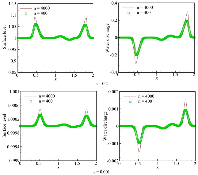
Figure 1. Surface level h + b (left) and water discharge hu (right) of the examples in section 4.3 at t = 0.2 s

图1. 在t = 0.2 s时,4.3节算例的表面水位h + b (左)和排水(右)

Figure 2. Free surface level h + b of the example in section 4.4 at t = 15 s (left) and t = 60 s (right)

图2. 在t = 15 s (左)和t = 60 s (右)时,在4.4节算例中的自由表面能级h + b

底部地形呈矩形

图2分别给出了 t = 15 s t = 60 s 时的数值解。显然目前格式得到了很好的数值解,与参考值和 [7] [9] [14] [51] 中的数值解一致。

4.5. 驼峰底部上的定常流

进一步,通过一个广泛应用的实例 [52] 对所提出的格式进行验证。实际上,本例基于给出的初始条件对跨临界流和次临界流进行数值模拟

h ( x , 0 ) = 0.33 mand u ( x , 0 ) = 0 m / s , x [ 0 , 25 ] m

底部地形呈驼峰状

b ( x ) = { ( 0.2 0.05 ( x 10 ) 2 ) mif 8 x 12m, 0 motherwise .

随后,我们在具有200个单元的网格上计算该例子,并计算至 t = 200 s ,施加不同的边界条件。此外,我们还展示了从 [53] 中得到的精确解,以便更好地进行比较。

l 算例A:无激波的跨临界流动

上游边界的流量 h u = 1.53 m 2 / s ,下游边界的水深 h = 0.66 m 图3中算例A结果表明,数值计算结果能够和实际结果吻合。

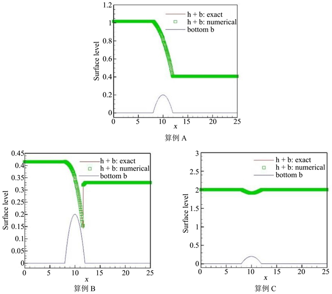
Figure 3. Surface level h + b in section 4.5 at t = 200

图3. 在t = 200时,第4.5节中的表面水位h + b

l 算例B:带激波的跨临界流动

上游边界的排水量 h u = 0.18 m 2 / s ,下游边界的水深 h = 0.33 m 图3中算例B结果表明,数值解与精确解具有良好的一致性,且无伪振荡。

l 算例C:亚临界流

其中,上游边界流量 h u = 0.18 m 2 / s ,下游边界水深 h = 2 m 图3中算例C表明,数值解与精确解拟合效果很好。

4.6. 台阶状底部上的溃坝问题

l 算例A:

此外,我们实现了一个来自 [54] [55] 的示例以及下面的初始条件

( h , u ) ( x , 0 ) = { ( 4 , 0 ) if x 0m, ( 1 , 0 ) otherwise, x [ 10 , 10 ] m

并超过一个台阶形状的底部

b ( x ) = { 0 mif x 0m , 1 motherwise .

随着时间的推移,这个数值算例产生了一个向左移动的稀疏薄和一个向右移动的激波。

l 算例B:

此外,我们使用不同的初始条件

( h , u ) ( x , 0 ) = { ( 4 , 5 ) mif x 0m, ( 1 , 0.9 ) motherwise , x [ 10 , 10 ] m

与上面相同的底部。随着时间推移,这个算例出现了两个向不同方向移动的冲击。

l 算例C:

初始条件由

( h , u ) ( x , 0 ) = { ( 0.75 , 9.49365 ) if x 0m, ( 1.10594 , 4.94074 ) otherwise , x [ 15 , 5 ] m

并超过一个台阶形状的底部

b ( x ) = { 0 mif x 0m, 0 .2 motherwise, (26)

l 算例D:

初始条件如下

( h , u ) ( x , 0 ) = { ( 0.75 , 1.35624 ) if x 0m, ( 1.10594 , 4.94074 ) otherwise , x [ 10 , 4 ] m

水体底部为(26)式。

图4给出了上述情况在同一网格上400个单元与精确网格的数值解,很明显,两者吻合较好。

Figure 4. Surface level h + b of the examples in Section 4.6

图4. 4.6节算例的表面h + b层

5. 结论

本文提出了一、二维非平坦地形浅水波方程的高阶精确熵稳定有限体积格式。首先,我们构造了二阶精确的well-balanced的半离散熵守恒有限体积格式,同时匹配物理通量的离散化和与非平底地形有关的源项的离散化。其次,以二阶精确熵守恒为基础,实现高阶精确均衡熵守恒格式。但熵守恒格式可能在间断附近产生杂散振荡,因此我们在熵守恒通量中加入适当的耗散项并构造满足半离散熵不等式的高阶半离散良好平衡的熵守恒格式。为了构造高阶耗散项,本文采用了基于缩放的熵变量的WENO重构。然后,采用高阶显式Runge-Kutta方法实现了时间区域的离散化。最后,大量的算例表明,本文所提出的格式保持了高阶精度,具有良好的平衡性,并能很好地捕捉到稳态下的小扰动。

致谢

本研究得到了山东省自然科学基金面上项目(No. ZR2021MA072)的资助。

NOTES

*通讯作者。

参考文献

[1] Bradford, S.F. and Sanders, B.F. (2002) Finite-Volume Model for Shallow Water Flooding of Arbitrary Topography. Journal of Hydraulic Engineering, 128, 289-298.
https://doi.org/10.1061/(ASCE)0733-9429(2002)128:3(289)
[2] Gottardi, G. and Venutelli, M. (2004) Central Scheme for the Two-Dimensional Dam-Break Flow Simulation. Advances in Water Resources, 27, 259-268.
https://doi.org/10.1016/j.advwatres.2003.12.006
[3] Vreugdenhil, C.B. (1995) Equations. In: Numerical Methods for Shallow-Water Flow, Water Science and Technology Library, Vol. 13, Springer, Dordrecht, 15-46.
https://doi.org/10.1007/978-94-015-8354-1_2
[4] Perthame, B. and Simeoni, C. (2001) A Kinetic Scheme for the Saint-Venant System with a Source Term. CALCOLO, 38, 201-231.
https://doi.org/10.1007/s10092-001-8181-3
[5] Xu. K. (2002) A Well-Balanced Gas-Kinetic Scheme for the Shallow-Water Equations with Source Terms. Journal of Computational Physics, 178, 533-562.
https://doi.org/10.1006/jcph.2002.7040
[6] Kurganov, A. and Levy, D. (2002) Central-Upwind Schemes for the Saint-Venant System. Mathematical Modelling and Numerical Analysis, 36, 397-425.
https://doi.org/10.1051/m2an:2002019
[7] Vukovic, S. and Sopta, L. (2002) ENO and WENO Schemes with the Exact Conservation Property for One-Dimen- sional Shallow Water Equations. Journal of Computational Physics, 179, 593-621.
https://doi.org/10.1006/jcph.2002.7076
[8] Vukovic, S., Crnjaric-Zic, N. and Sopta, L. (2004) WENO Schemes for Balance Laws with Spatially Varying Flux. Journal of Computational Physics, 199, 87-109.
https://doi.org/10.1016/j.jcp.2004.02.002
[9] Xing, Y.L. and Shu, C.-W. (2005) High Order Finite Difference WENO Schemes with the Exact Conservation Property for the Shallow Water Equations. Journal of Computational Physics, 208, 206-227.
https://doi.org/10.1016/j.jcp.2005.02.006
[10] Noelle, S., Pankratz, N., Puppo, G. and Natvig, J. (2006) Well-Balanced Finite Volume Schemes of Arbitrary Order of Accuracy for Shallow Water Flows. Journal of Computa-tional Physics, 213, 474-499.
https://doi.org/10.1016/j.jcp.2005.08.019
[11] Xing, Y.L. and Shu, C.-W. (2006) High Order Well-Balanced Finite Volume WENO Schemes and Discontinuous Galerkin Methods for a Class of Hyperbolic Systems with Source Terms. Journal of Computational Physics, 214, 567-598.
https://doi.org/10.1016/j.jcp.2005.10.005
[12] Noelle, S., Xing, Y. and Shu, C.-W. (2007) High-Order Well-Balanced Finite Volume WENO Schemes for Shallow Water Equation with Moving Water. Journal of Computational Physics, 226, 29-58.
https://doi.org/10.1016/j.jcp.2007.03.031
[13] Li, G., Lu, C. and Qiu, J. (2012) Hybrid Well-Balanced WENO Schemes with Different Indicators for Shallow Water Equations. Journal of Scientific Computing, 51, 527-559.
https://doi.org/10.1007/s10915-011-9520-4
[14] Li, G., Caleffi, V. and Qi, Z.K. (2015) A Well-Balanced Finite Difference WENO Scheme for Shallow Water Flow Model. Applied Mathematics and Computation, 265, 1-16.
https://doi.org/10.1016/j.amc.2015.04.054
[15] Zhu, Q., Gao, Z., Don, W.S. and Lv, X. (2017) Well-Balanced Hy-brid Compact-WENO Scheme for Shallow Water Equations. Applied Numerical Mathematics, 112, 65-78.
https://doi.org/10.1016/j.apnum.2016.10.001
[16] Li, J.J., Li, G., Qian, S.G. and Gao, J.M. (2021) High-Order Well-Balanced Finite Volume WENO Schemes with Conservative Variables Decomposition for Shallow Water Equa-tions. Advances in Applied Mathematics and Mechanics, 13, 827-849.
https://doi.org/10.4208/aamm.OA-2020-0138
[17] Caleffi, V. (2011) A New Well-Balanced Hermite Weighted Essentially Non-Oscillatory Scheme for Shallow Water Equations. International Journal for Numerical Methods in Flu-ids, 67, 1135-1159.
https://doi.org/10.1002/fld.2410
[18] Russo, G. (2000) Central Schemes for Balance Laws. In: Freistühler, H. and Warnecke, G., Eds., Hyperbolic Problems: Theory, Numerics, Applications, ISNM International Se-ries of Numerical Mathematics, Vol. 141, Birkhäuser, Basel, 821-829.
https://doi.org/10.1007/978-3-0348-8372-6_35
[19] Touma, R. and Khankan, S. (2012) Well-Balanced Unstag-gered Central Schemes for One and Twodimensional Shallow Water Equation Systems. Applied Mathematics and Com-putation, 218, 5948-5960.
https://doi.org/10.1016/j.amc.2011.11.059
[20] Dong, J. (2020) A Robust Central Scheme for the Shallow Water Flows with an Abrupt Topography Based on Modified Hydrostatic Reconstructions. Mathematical Methods in the Ap-plied Sciences, 43, 9024-9045.
https://doi.org/10.1002/mma.6597
[21] Dong, J. and Li, D.F. (2021) Well-Balanced Nonstaggered Central Schemes Based on Hydrostatic Reconstruction for the Shallow Water Equations with Coriolis Forces and Topography. Mathemat-ical Methods in the Applied Sciences, 44, 1358-1376.
https://doi.org/10.1002/mma.6835
[22] Ern, A., Piperno, S. and Djadel, K. (2008) A Well-Balanced Runge-Kutta Discontinuous Galerkin Method for the Shallow-Water Equations with Flooding and Drying. International Journal for Numerical Methods in Fluids, 58, 1-25.
https://doi.org/10.1002/fld.1674
[23] Xing, Y. (2014) Exactly Well-Balanced Discontinuous Galerkin Methods for the Shallow Water Equations with Moving Water Equilibrium. Journal of Computational Physics, 257, 536-553.
https://doi.org/10.1016/j.jcp.2013.10.010
[24] Li, G., Song, L.N. and Gao. J.M. (2018) High Order Well-Balanced Discontinuous Galerkin Methods Based on Hydrostatic Reconstruction for Shallow Water Equations. Journal of Com-putational and Applied Mathematics, 340, 546-560.
https://doi.org/10.1016/j.cam.2017.10.027
[25] Vignoli, G., Titarev, V.A. and Toro, E.F. (2008) ADER Schemes for the Shallow water Equations in Channel with Irregular Bottom Elevation. Journal of Computational Physics, 227, 2463-2480.
https://doi.org/10.1016/j.jcp.2007.11.006
[26] Navas-Montilla, A. and Murillo, J. (2015) Energy Balanced Numer-ical Schemes with very High Order. The Augmented Roe Flux ADER Scheme. Application to the Shallow Water Equa-tions. Journal of Computational Physics, 290, 188-218.
https://doi.org/10.1016/j.jcp.2015.03.002
[27] Gassner, G.J., Winters A.R. and Kopriva, D.A. (2016) A Well Balanced and Entropy Conservative Discontinuous Galerkin Spec-tral Element Method for the Shallow Water Equations. Applied Mathematics and Computation, 272, 291-308.
https://doi.org/10.1016/j.amc.2015.07.014
[28] Berthon, C. and Chalons, C. (2016) A Fully Well-Balanced, Posi-tive and Entropy-Satisfying Godunov-Type Method for the Shallow-Water Equations. Mathematics of Computation, 85, 1281-1307.
https://doi.org/10.1090/mcom3045
[29] Li, D.F. and Dong, J. (2022) A Robust Hybrid Unstaggered Central and Godunov-Type Scheme for Saint-Venant-Exner Equations with Wet/Dry Fronts. Computers & Fluids, 235, Article ID: 105284.
https://doi.org/10.1016/j.compfluid.2021.105284
[30] Yuan, X.H. (2018) A Well-Balanced Element-Free Galerkin Method for the Nonlinear Shallow Water Equations. Applied Mathematics and Computation, 331, 46-53.
https://doi.org/10.1016/j.amc.2018.01.061
[31] Liu, X., Mohammadian, A., Kurganov, A. and Sedano, J.A.I. (2015) Well-Balanced Central-Upwind Scheme for a Fully Coupled Shallow Water System Modeling Flows over Erodible Bed. Journal of Computational Physics, 300, 202-218.
https://doi.org/10.1016/j.jcp.2015.07.043
[32] Chertock, A., Kurganov, A. and Wu, T. (2020) Operator Splitting Based Central-Upwind Schemes for Shallow Water equations with Moving Bottom Topography. Communications in Mathematical Sciences, 18, 2149-2168.
https://doi.org/10.4310/CMS.2020.v18.n8.a3
[33] Li, G., Li, J.J., Qian, S.G. and Gao, J.M. (2021) A Well-Balanced ADER Discontinuous Galerkin Method Based on Differential Transformation Procedure for Shallow Water Equations. Applied Mathematics and Computation, 395, Article ID: 125848.
https://doi.org/10.1016/j.amc.2020.125848
[34] Duan, J.M. and Tang. H.Z. (2021) High-Order Accurate Entropy Stable Finite Difference Schemes for the Shallow Water Magnetohydrodynamics. Journal of Computational Physics, 431, Article ID: 110136.
https://doi.org/10.1016/j.jcp.2021.110136
[35] Winters, A.R. and Gassner, G.J. (2015) A Comparison of Two En-tropy Stable Discontinuous Galerkin Spectral Element Approximations for the Shallow Water Equations with Non-Constant Topography Author Links Open Overlay Panel. Journal of Computational Physics, 301, 357-376.
https://doi.org/10.1016/j.jcp.2015.08.034
[36] Wintermeyer, N., Winters, A.R., Gassner, G.J. and Kopriva, D.A. (2017) An Entropy Stable Nodal Discontinuous Galerkin Method for the Two Dimensional Shallow Water Equations on Unstructured Curvilinear Meshes with Discontinuous Bathymetry. Journal of Computational Physics, 340, 200-242.
https://doi.org/10.1016/j.jcp.2017.03.036
[37] Wintermeyer, N., Winters, A.R., Gassner, G.J. and Warburton, T. (2018) An entropy stable discontinuous Galerkin method for the Shallow Water Equations on Curvilinear Meshes with Wet/Dry Fronts Accelerated by GPUs. Journal of Computational Physics, 375, 447-480.
https://doi.org/10.1016/j.jcp.2018.08.038
[38] Wen, X., Don, W.S., Gao, Z. and Xing, Y.L. (2020) Entropy Stable and Well-Balanced Discontinuous Galerkin Methods for the Nonlinear Shallow Water Equations Journal of Scientific Computing, 83, Article No. 66.
https://doi.org/10.1007/s10915-020-01248-3
[39] Liu, Q.S., Liu, Y.Q. and Feng, J.H. (2019) The Scaled Entropy Variables Reconstruction for Entropy Stable Schemes with Application to Shallow Water Equations. Computers & Fluids, 192, Article ID: 104266.
https://doi.org/10.1016/j.compfluid.2019.104266
[40] Fjordholm, U.S., Mishra, S. and Tadmor, E. (2011) Well-Balanced and Energy Stable Schemes for the Shallow Water Equations with Discontinuous Topography Journal of Computational Physics, 230, 5587-5609.
https://doi.org/10.1016/j.jcp.2011.03.042
[41] Fjordholm, U.S., Mishra, S. and Tadmor, E. (1987) The Numerical Viscosity of Entropy Stable Schemes for Systems of Conservation Laws. I. Mathematics of Computation, 49, 91-103.
https://doi.org/10.1090/S0025-5718-1987-0890255-3
[42] Lefloch, P.G., Mercier, J.M. and Rohde, C. (2002) Fully Discrete Entropy Conservative Schemes of Arbitrary Order. SIAM Journal on Numerical Analysis, 40, 1968-1992.
https://doi.org/10.1137/S003614290240069X
[43] Fjordholm, U.S., Mishra, S. and Tadmor, E. (2012) Arbitrarily High-Order Accurate Entropy Stable Essentially Non- Oscillatory Schemes for Systems of Conservation Laws. SIAM Journal on Numerical Analysis, 50, 544-573.
https://doi.org/10.1137/110836961
[44] Fjordholm, U.S., Mishra, S. and Tadmor, E. (2013) ENO Reconstruction and ENO Interpolation Are Stable. Foundations of Computational Mathematics, 13, 139-159.
https://doi.org/10.1007/s10208-012-9117-9
[45] Shu, C.-W. (1997) Essentially Non-Oscillatory and Weighted Es-sentially Non-Oscillatory Schemes for Hyperbolic Conservation Laws. NASA/CR-97-206253, ICASE Report No. 97-65.
[46] Shu, C.-W. (2009) High Order Weighted Essentially Nonoscillatory Schemes for Convection Dominated Problems. SIAM Review, 51, 82-126.
https://doi.org/10.1137/070679065
[47] Shu, C.-W. (2016) High Order WENO and DG Methods for Time-Dependent Convectiondominated PDEs: Abrief Survey of Several Recent Develop-ments. Journal of Computational Physics, 316, 598-613.
https://doi.org/10.1016/j.jcp.2016.04.030
[48] Biswas, B. and Dubey, R.K. (2018) Low Dissipative Entropy Stable Schemes Using Third Order WENO and TVD Reconstructions. Advances in Computational Mathematics, 44, 1153-1181.
https://doi.org/10.1007/s10444-017-9576-2
[49] Shu, C.-W. and Osher, S. (1998) Efficient Implemen-tation of Essentially Non-Oscillatory Shockcapturing Schemes. Journal of Computational Physics, 77, 439-471.
https://doi.org/10.1016/0021-9991(88)90177-5
[50] LeVeque, R.J. (1998) Balancing Source Terms and Flux Gra-dient on High-Resolution Godunov Methods: The Quasi-Steady Wave-Propagation Algorithm. Journal of Computation-al Physics, 146, 346-365.
https://doi.org/10.1006/jcph.1998.6058
[51] Xing, Y.L. and Shu, C.-W. (2006) A New Approach of High Order Well-Balanced Finite Volume WENO Schemes and Discontinuous Galerkin Methods for a Class of Hyperbolic Systems with Source Terms. Communications in Computational Physics, 1, 100-134.
[52] Vazquez-Cendon, M.E. (1999) Im-proved Treatment of Source Terms in Upwind Schemes for the Shallow Water Equations in Channels with Irregular Geometry. Journal of Computational Physics, 148, 497-526.
https://doi.org/10.1006/jcph.1998.6127
[53] Goutal, N. and Maurel, F. (1997) Proceedings of the Second Work-shop on Dam-Break Wave Simulation. Technical Report HE-43/97/016/A, Electricité de France, Département Laboratoire National d’Hydraulique, Groupe Hydraulique Fluviale.
[54] Bermudez, A. and Vazquez, M.E. (1994) Upwind Methods for Hyperbolic Conservation Laws with Source Terms. Computers & Fluids, 23, 1049-1071.
https://doi.org/10.1016/0045-7930(94)90004-3
[55] Alcrudo, F. and Benkhaldoun, F. (2001) Exact Solution to the Riemann Problem of the Shallow Water Euqaionts with a Bottom Step. Computers & Fluids, 30, 643-671.
https://doi.org/10.1016/S0045-7930(01)00013-5