基于流体静力学重构的天然气流动模型的Well-Balanced间断伽辽金方法

A Well-Balanced Discontinuous Galerkin Method Based on Hydrostatic Reconstruction for Real Gas in Pipelines

摘要: 在本文研究中，我们针对天然气科学与工程领域中天然气流动模型建立了高阶well-balanced间断伽辽金有限元方法。管道中的天然气流动模型精确保持速度为零的定常状态。为了从数值角度上保持该定常状态，我们提出了well-balanced数值流通量以及一种崭新的源项离散，最终建立了高阶间断伽辽金有限元方法。此方法能够在离散状态下精确保持速度为零的定常状态。严格的理论分析以及广泛的数值结果均验证了本方法保持良好的特性。此外，数值实验还验证了该方法对于小扰动具有精确捕捉能力和良好的分辨率。我们相信该方法在天然气科学与工程领域中具有潜在应用前景。

Abstract: In this research, we propose high order well-balanced discontinuous Galerkin methods for real gas in pipelines in the fields of the natural gas science and engineering. The model of real gas in pipelines preserves the steady state exactly. In order to maintain the steady state at the discrete level, we propose to construct the well-balanced numerical fluxes as well as a novel source term approximation. In this article, by means of hydrostatic reconstruction, we build a high order discontinuous Galerkin method, which exactly preserves the steady state, and is characterized by a discharge equal to zero (analogue to hydrostatic equilibrium). Rigorous theoretical analysis as well as extensive numerical results, all validate that the current method preserves the well-balanced property. In addition, numerical experiments are carried out to validate the ability to capture small perturbation of steady state, and high resolutions. We believe that the resulting method has potential applications in the fields of natural gas science and engineering.

1. 引言

针对管道中天然气流动的数学建模以及数值模拟是规划和运行天然气输送网络中的一个重要课题，具有实际的应用价值。管道中天然气流动过程可以经由带有源项的可压缩欧拉方程来刻画。关于该数学模型的研究可以帮助优化管道设计，进而节省天然气输运过程中由于自耗引起的运行成本。此外，由于管道中天然气流动过程是一个高度非线性的复杂过程，导致理论分析超级困难，实验研究耗时耗力。然而，科学计算可以帮助工程师利用计算机模拟再现天然气在管道中的流动过程，帮助呈现摩擦力、温度的分布，从而节约时间，节约成本，具有较高的经济效益。

近年来，由于高速计算机的迅猛发展，借助于高阶数值方法针对管道中天然气流动过程进行数值模拟在天然气输送网络的规划与运行中获得了广泛应用 [1] [2] [3]。截至目前，大多数关于这一课题的研究和计算程序都是处理定常状态的情况。

在实际问题中，管道相对于基准面的高度根据地形变化而变化是非常常见的，这个现状导致了气体流动模型中源项的产生。这种情况类似于水动力学中由于水体底部不平而导致的几何源项 [4]。在实际的高压输气网络中，气体表现为真实气体，因此需要考虑可压缩因素对理想气体方程进行修正。综上所述，运输管道中天然气流动的数学描述可以通过如下控制方程来刻画 [5]：

$\{\begin{array}{l}{\rho }_t+{\left(\rho u\right)}_x=0\\ {\left(\rho u\right)}_t+{\left(\rho u^2+p\right)}_x=-\frac{\lambda }{2D}\rho \left|u\right|u-g\rho h_x\\ E_t+{\left(\left(E+p\right)u\right)}_x=\frac{4\beta }{D}\left({\theta }_{ext}-\theta \right)-g\rho u{h}_x\end{array}$ (1)

其中， $\rho ,u,p$ 分别表示流体密度、速度和压力。E是总能量，包括流体的动能和内能。D表示管道直径。符号 $\theta$ 和 ${\theta }_{ext}$ 分别代表平均温度和外部温度。 $\beta$ 为传热系数。为了闭合这个方程组，我们使用理想气体定律

$p=\left(\gamma -1\right)\rho e=\left(\gamma -1\right)\left(E-\frac{1}{2}\rho u^2\right),$

其中 $\gamma$ 是绝热比。

从数学的角度来看，方程组(1)属于双曲平衡律，其主要特征是保持速度为零的定常状态(即解关于时间的导数为零)

$u=0,\theta ={\theta }_{ext}$ (2)

换言之，物理流通量非零，且其梯度可以被源项精确平衡掉。在离散状态下，能够保持流通量梯度和源项之间精确平衡的数值方法是备受欢迎的。然而，上述平衡既不是常数，也不是多项式，这给高阶数值方法的构造带来了极大挑战。一般情况下，简单直接的源项离散方式会破坏掉这个微妙的平衡状态，容易导致虚假震荡，严重的会致使程序崩溃。此外，网格加细策略仅能降低震荡幅度，无法彻底消除震荡。更进一步，网格加细策略计算成本太高，尤其针对高维问题，不利于实际问题。Greenberg联同合作者 [6] [7] 原创性地提出了well-balanced方法，该方法在离散状态下精确保持流通量梯度与源项之间的平衡。换句话说，well-balanced方法能够保持定常状态至机器精度。此外，较之non-well-balanced方法，well-balanced方法可以基于较粗网格有效捕捉关于定常状态的小扰动 [8] [9]，进而节约计算成本，更加适应实际问题的需求。

在本研究中，我们针对保持定常状态的天然气流动模型构造了高阶well-balanced间断伽辽金(Discontinuous Galerkin，简称DG)方法。为了实现该well-balanced性质，我们首先给出了源项的重新表达，进而建立了一种崭新的源项离散以及分解算法。最终所得到的DG方法既保持了well-balanced性质，同时针对间断解保持陡峭的间断过渡。

DG方法是一种以分段多项式空间作为试探解和检验函数空间的有限元方法。DG方法结合了有限元方法和有限体积方法的优点(见 [10] [11] 的简要历史回顾)，拥有高阶精度、易于并行计算、hp自适应的灵活性、方便处理复杂边界和任意几何形状，从而使之得到了广泛应用 [12] [13] [14]。基于上述优点，从21世纪初至今，DG方法在计算流体力学领域中获得了成功应用 [15] - [25]。据我们所知，这将是首次将DG方法用于管道中天然气流动的数值模拟当中。

本文的组织结构如下。在第2节中，我们详细介绍了well-balanced的DG方法。然后，在第三节中，我们进行了一些数值实验来验证所得到方法的性能。结论在第四章给出。

2. 管道内天然气流体模型的well-balanced DG法的建立

首先，将空间区域剖分为N个一致单元，其中 $I_j=\left[x_{j-\frac{1}{2}},x_{j+\frac{1}{2}}\right],j=1,2,\cdots ,N$。这里 $x_j=\frac{1}{2}\left(x_{j-\frac{1}{2}}+x_{j+\frac{1}{2}}\right)$ 表示单元中心， ${\tau }_j=x_{j+\frac{1}{2}}-x_{j-\frac{1}{2}}$ 表示网格尺寸， $\tau ={\max }_{1\le j\le N}{\tau }_j$ 表示最大网格尺寸。近似解空间 $V_{\tau }^k$ 被定义为每个单元 $I_j$ 上次数小于等于k的分段多项式集合：

$V_{\tau }^k=\left\{\phi :{\phi |}_{I_j}\in P^k\left(I_j\right),j=1,2,\cdots ,N\right\}.$ (3)

注意在 $V_{\tau }^k$ 中的多项式可以在单元界面处保持间断。

在DG方法的框架下，我们取 $U_{\tau }\in V_{\tau }^k$ 作为对精确解U的数值近似。此外，我们分别用 $U_{\tau ,j+\frac{1}{2}}^{-}$ 和 $U_{\tau ,j+\frac{1}{2}}^{+}$ 表示数值解 $U_{\tau }$ 在单元内分别从左单元 $I_j$ 和右单元 $I_{j+1}$ 的极限值。更进一步，我们用 $\left\{U\right\}\left(x_{j+\frac{1}{2}}\right)=\frac{1}{2}\left(U_{\tau ,\frac{1}{2}}^{-}+U_{\tau ,\frac{1}{2}}^{+}\right)$ 表示 $U_{\tau }$ 在单元界面 $x_{j+\frac{1}{2}}$ 处两侧值得算术平均值。

当方程处于定常状态(2)时，控制方程(1)中的动量方程满足

$p_x=-g\rho h_x.$ (4)

此外，对于理想气体，我们有等式 $P=R{\theta }_{ext}\rho$，其中R为气体常数。我们可以把(4)等价地改写为

$R{\theta }_{ext}{\rho }_x=-g\rho h_x.$

将上式在区间 $\left[0,x\right]$ 上进行积分，并通过简单代数运算，可以将密度 ${\rho }_x$ 和压力 $p_x$ 分别表示为

$\begin{array}{l}\rho \left(x\right)=\rho \left(0\right)\exp \left(-\frac{g}{R{\theta }_{ext}}\left(h\left(x\right)-h\left(0\right)\right)\right),\\ p\left(x\right)=R{\theta }_{ext}\rho \left(0\right)\exp \left(-\frac{g}{R{\theta }_{ext}}\left(h\left(x\right)-h\left(0\right)\right)\right).\end{array}$ (5)

因此，控制方程(1)可以等价地重新表述为：

$\{\begin{array}{l}{\rho }_t+{\left(\rho u\right)}_x=0,\\ {\left(\rho u\right)}_t+{\left(\rho u^2+p\right)}_x=-\frac{\lambda }{2D}\rho \left|u\right|u+R{\theta }_{ext}\rho \frac{\exp {\left(-\frac{g}{R{\theta }_{ext}}\left(h\left(x\right)-h\left(0\right)\right)\right)}_x}{\exp \left(-\frac{g}{R{\theta }_{ext}}\left(h\left(x\right)-h\left(0\right)\right)\right)},\\ E_t+{\left(\left(E+p\right)u\right)}_x=\frac{4\beta }{D}\left({\theta }_{ext}-\theta \right)-g\rho u{h}_x,\end{array}$ (6)

或者如下紧致形式

$U_t+F{\left(U\right)}_x=S,$ (7)

其中 $U={\left(\rho ,\rho u,E\right)}^{\text{T}}$ 表示守恒变量， $F\left(U\right)$ 表示物理通量，S为源项。

在DG方法的框架下，控制方程(1)的标准半离散DG方法定义如下：对于任何测试函数 $\varphi \in V_T^k$，数值解 $U_t$ 满足以下弱形式

${\displaystyle {\int }_{I_j}{\left(U_{\tau }\right)}_t\varphi \text{d}x}-{\displaystyle {\int }_{I_j}F\left(U_{\tau }\right){\varphi }_x\text{d}x}+{\hat{F}}_{j+\frac{1}{2}}\varphi \left(x_{j+\frac{1}{2}}^{-}\right)-{\hat{F}}_{j-\frac{1}{2}}\varphi \left(x_{j-\frac{1}{2}}^{+}\right)={\displaystyle {\int }_{I_j}S\varphi \text{d}x}$ (8)

其中 ${\hat{F}}_{j+\frac{1}{2}}=\hat{f}\left(U_{\tau ,j+\frac{1}{2}}^{-},U_{\tau ,j+\frac{1}{2}}^{+}\right)$ 表示单元界面 $x_{j+\frac{1}{2}}$ 处的数值流通量，用来近似物理流通量 $F\left(U\left(x_{j+\frac{1}{2}},t\right)\right)$。本文中，我们采用简单高效的Lax-Friedrichs流通量，即

$\hat{f}\left(a_1,a_2\right)=\frac{1}{2}\left(F\left(a_1\right)+F\left(a_2\right)-\alpha \left(a_2-a_1\right)\right),$ (9)

其中 $\alpha$ 表示雅克比矩阵 $\frac{\partial F\left(U\right)}{\partial U}$ 的特征值的绝对值的最大值。

2.1. Well-balanced数值流通量的构造

设计well-balanced DG方法的关键步骤在于构造well-balanced数值流通量 ${\hat{F}}_{j+\frac{1}{2}}$。式(9)中的数值黏性项 $\alpha \left(a_2-a_1\right)$ 是针对双曲守恒律稳定性的必要选择。然而，它会破坏数值方法的well-balanced性能。因此，我们对(9)中原有数值流通量做如下修改

${\hat{F}}_{j+\frac{1}{2}}=\frac{1}{2}\left[F\left(U_{\tau ,j+\frac{1}{2}}^{-}\right)+F\left(U_{\tau ,j+\frac{1}{2}}^{+}\right)-\alpha \left({\tilde{U}}_{\tau ,j+\frac{1}{2}}^{+}-{\tilde{U}}_{\tau ,j+\frac{1}{2}}^{-}\right)\right],$ (10)

其中 $\tilde{U}=\frac{U}{\rho }$。在定常状态下， $\tilde{U}$ 退化为常数，故数值粘性项 $\alpha \left({\tilde{U}}_{\tau ,j+\frac{1}{2}}^{+}-{\tilde{U}}_{\tau ,j+\frac{1}{2}}^{-}\right)$ 相应地转变为零。因此，粘度项的影响褪变为零。所以，针对定常状态数值流通量相应地演变成如下简单形式

${\hat{F}}_{j+\frac{1}{2}}=\frac{1}{2}\left[F\left(U_{\tau ,j+\frac{1}{2}}^{-}\right)+F\left(U_{\tau ,j+\frac{1}{2}}^{+}\right)\right].$ (11)

2.2. 一种新的源项离散

接下来，我们针对源项提出一种新的离散方式。为了便于描述，首先定义如下符号

$b\left(x\right)=\exp \left(-\frac{g}{R{\theta }_{ext}}\left(h\left(x\right)-h\left(0\right)\right)\right),$ (12)

从而，我们得到等式

$-g\rho h_x=R{\theta }_{ext}\frac{\rho }{b}{b}_x$ (13)

接下来，我们将第二个方程中源项的积分分裂为

$\begin{array}{c}{\displaystyle {\int }_{I_j}{S}^{\left|2\right|}\varphi \text{d}x}=-\frac{\lambda }{2D}{\displaystyle {\int }_{I_j}\rho \left|u\right|u\varphi \text{d}x}+R{\theta }_{ext}{\displaystyle {\int }_{I_j}\frac{\rho }{b}{b}_x\varphi \text{d}x}\\ =-\frac{\lambda }{2D}{\displaystyle {\int }_{I_j}\rho \left|u\right|u\varphi \text{d}x}+R{\theta }_{ext}{\displaystyle {\int }_{I_j}\left(\frac{\rho }{b}-\frac{\rho \left(x_j\right)}{b\left(x_j\right)}+\frac{\rho \left(x_j\right)}{b\left(x_j\right)}\right)b_x\varphi \text{d}x}\\ =-\frac{\lambda }{2D}{\displaystyle {\int }_{I_j}\rho \left|u\right|u\varphi \text{d}x}+R{\theta }_{ext}{\displaystyle {\int }_{I_j}\left(\frac{\rho }{b}-\frac{\rho \left(x_j\right)}{b\left(x_j\right)}\right)b_x\varphi \text{d}x}\\ +R{\theta }_{ext}\frac{\rho \left(x_j\right)}{b\left(x_j\right)}\left(\left(b\left(x_{j+\frac{1}{2}}\right)\varphi \left(x_{j+\frac{1}{2}}^{-}\right)-b\left(x_{j-\frac{1}{2}}\right)\varphi \left(x_{j-\frac{1}{2}}^{+}\right)\right)-{\displaystyle {\int }_{I_j}{b}_x\varphi \text{d}x}\right)\end{array}$

我们现在将函数 $b\left(x\right)$ 投影到空间 $V_{\tau }^k$ 中，利用 $L^2$ 投影得到多项式 $b_{\tau }\left(x\right)$。从而，我们得到对于第二个方程中源项的数值离散

$\begin{array}{c}{\displaystyle {\int }_{I_j}{S}^{\left|2\right|}\varphi \text{d}x}\approx -\frac{\lambda }{2D}{\displaystyle {\int }_{I_j}{\rho }_{\tau }\left|u_{\tau }\right|u_{\tau }\varphi \text{d}x}+R{\theta }_{ext}{\displaystyle {\int }_{I_j}\left(\frac{{\rho }_{\tau }}{b_{\tau }}-\frac{{\rho }_{\tau }\left(x_j\right)}{b_{\tau }\left(x_j\right)}\right){\left(b_{\tau }\right)}_x\varphi \text{d}x}\\ +R{\theta }_{ext}\frac{{\rho }_{\tau }\left(x_j\right)}{b_{\tau }\left(x_j\right)}\left(\left\{b_{\tau }\right\}\left(x_{j+\frac{1}{2}}\right)\varphi \left(x_{j+\frac{1}{2}}^{-}\right)-\left\{b_{\tau }\right\}b\left(x_{j-\frac{1}{2}}\right)\varphi \left(x_{j-\frac{1}{2}}^{+}\right)\right)\\ -R{\theta }_{ext}\frac{{\rho }_{\tau }\left(x_j\right)}{b_{\tau }\left(x_j\right)}{\displaystyle {\int }_{I_j}{b}_{\tau }{\varphi }_x\text{d}x}\end{array}$ (14)

其中 $\rho$ 和b分别用 ${\rho }_{\tau }$ 和 $b_{\tau }$ 代替，另外 $b_{\tau }$ 的单元界面值用 $b_{\tau }$ 所在的单元界面两侧值的算术平均值 $\left\{b_{\tau }\right\}$ 来代替。此外，对于第三个方程中的源项，我们采用具有足够高精度的高斯求积公式来逼近。

2.3. Well-balanced DG方法

上述操作导出关于带有源项的欧拉方程(1)的well-balanced DG方法，详见如下命题所述

命题1：结合式(10)和式(14)，半离散DG方法(8)对于定常状态(2)保持well-balanced性质。

证明：在定常状态(2)下，我们首先拥有

${\rho }_{\tau }=\rho \left(0\right)b_{\tau },u_{\tau }=0,p_{\tau }=R{\theta }_{ext}\rho \left(0\right)b_{\tau }.$ (15)

由于 $u=0$，第一、三方程中的流通量和源项均都变为零。因此，第一个和第三个方程显然保持精确平衡。接下来，聚焦于第二个方程。对于动量方程，联合式(5)和式(12)得到以下等式

$\frac{{\rho }_{\tau }\left(x_j\right)}{b_{\tau }\left(x_j\right)}=\frac{{\rho }_{\tau }\left(x\right)}{b_{\tau }\left(x\right)}\equiv \rho \left(0\right).$ (16)

由于式(15)、(16)，源项离散(14)相应地变为

$\begin{array}{c}{\displaystyle {\int }_{I_j}{S}^{\left|2\right|}\varphi \text{d}x}\approx R{\theta }_{ext}\frac{\rho \left(x_j\right)}{b\left(x_j\right)}\left(\left\{b_{\tau }\right\}\left(x_{j+\frac{1}{2}}\right)\varphi \left(x_{j+\frac{1}{2}}^{-}\right)-\left\{b_{\tau }\right\}b\left(x_{j-\frac{1}{2}}\right)\varphi \left(x_{j-\frac{1}{2}}^{+}\right)-{\displaystyle {\int }_{I_j}{b}_{\tau }{\varphi }_x\text{d}x}\right)\\ \approx R{\theta }_{ext}\rho \left(0\right)\left(\left\{b_{\tau }\right\}\left(x_{j+\frac{1}{2}}\right)\varphi \left(x_{j+\frac{1}{2}}^{-}\right)-\left\{b_{\tau }\right\}b\left(x_{j-\frac{1}{2}}\right)\varphi \left(x_{j-\frac{1}{2}}^{+}\right)-{\displaystyle {\int }_{I_j}{b}_{\tau }{\varphi }_x\text{d}x}\right)\end{array}$ (17)

另外，由于 $u=0$，第二个物理流通量 $F^{\left|2\right|}\left(U\right)=\rho u^2+p$ 退化为p。借助于式(10)以及等式 $p_{\tau }=R{\theta }_{ext}\rho \left(0\right)b_{\tau }$，式(8)中针对第二个方程中流通量梯度的数值逼近转化为

$\begin{array}{l}{\hat{F}}_{j+\frac{1}{2}}^{\left|2\right|}\varphi \left(x_{j+\frac{1}{2}}^{-}\right)-{\hat{F}}_{j-\frac{1}{2}}^{\left|2\right|}\varphi \left(x_{j-\frac{1}{2}}^{+}\right)-{\displaystyle {\int }_{I_j}F\left(U_{\tau }\right){\varphi }_x\text{d}x}\\ =R{\theta }_{ext}\rho \left(0\right)\left({\left\{b_{\tau }\right\}}_{j+\frac{1}{2}}\varphi \left(x_{j+\frac{1}{2}}^{-}\right)-{\left\{b_{\tau }\right\}}_{j-\frac{1}{2}}\varphi \left(x_{j-\frac{1}{2}}^{+}\right)-R{\theta }_{ext}\rho \left(0\right){\displaystyle {\int }_{I_j}{b}_{\tau }{\varphi }_x\text{d}x}\right)\\ =R{\theta }_{ext}\rho \left(0\right)\left({\left\{b_{\tau }\right\}}_{j+\frac{1}{2}}\varphi \left(x_{j+\frac{1}{2}}^{-}\right)-{\left\{b_{\tau }\right\}}_{j-\frac{1}{2}}\varphi \left(x_{j-\frac{1}{2}}^{+}\right)-{\displaystyle {\int }_{I_j}{b}_{\tau }{\varphi }_x\text{d}x}\right)\end{array}$ (18)

比较式(17)与(18)，我们发现针对流通量梯度的逼近与针对源项的逼近相互抵消掉的，这导致所得到的DG方法保持所期待的well-balanced性质。

在取得了数值流通量(10)和源项离散(14)之后，我们获得了半离散DG方法(8)的简洁形式

$\frac{\text{d}{U}_{\tau }}{\text{d}t}=\mathcal{L}\left(U_{\tau }\right).$ (19)

实际上，式(19)是一常微分方程，其中 $\mathcal{L}\left(U_{\tau }\right)$ 表示空间算子，包含了针对流通量梯度和源项的离散。对于常微分方程(19)的向前时间推进，我们采用经典的三阶 Runge-Kutta方法 [26]：

$\begin{array}{l}{U}_{\tau }^{\left(1\right)}=U_{\tau }^n+\Delta t\mathcal{L}\left(U_{\tau }^n\right),\\ U_{\tau }^{\left(2\right)}=\frac{3}{4}{U}_{\tau }^n+\frac{1}{4}\left(U_{\tau }^{\left(1\right)}+\Delta t\mathcal{L}\left(U_{\tau }^{\left(1\right)}\right)\right),\\ U_{\tau }^{n+1}=\frac{1}{3}{U}_{\tau }^n+\frac{2}{3}\left(U_{\tau }^{\left(2\right)}+\Delta t\mathcal{L}\left(U_{\tau }^{\left(2\right)}\right)\right).\end{array}$ (20)

3. 数值结果

在本节中，我们将通过不同算例来测试所提出的三阶DG方法的性能。我们采用三阶Runge-Kutta方法(20)，并在整个计算过程中取重力常数g为9.812，为了保持数值稳定性取 $CFL=0.18$。

3.1. 测试well-balanced性质

通过第一个数值算例，我们来测试所提方法的well-balanced性质。初始条件满足如下定常状态

$\begin{array}{l}\rho \left(x,0\right)=\rho \left(0\right)\exp \left(-\frac{g}{R{\theta }_{ext}}\left(h\left(x\right)-h\left(0\right)\right)\right),\\ u\left(x,0\right)=0,\\ p\left(x,0\right)=R{\theta }_{ext}\rho \left(0\right)\exp \left(-\frac{g}{R{\theta }_{ext}}\left(h\left(x\right)-h\left(0\right)\right)\right),\end{array}$

其中计算区域为 $\left[0,40\right]$，取参数分别为 $R=480$， $\rho \left(0\right)=1$， $\theta \left(x\right)={\theta }_{ext}=288.15$， $h\left(x\right)=1000\sin \left(\pi x/40\right)$。

然后，分别基于包含100和200个单元的均匀网格上，将该算例计算至时刻 $t=0.25$。为了表明即使在舍入误差存在的前提下，该方法也能保持well-balanced性质，分别借助于单精度和双精度实施了计算，并将 $\rho ,\rho u,E$ 在 $t=0.25$ 时刻与初始时刻的 $L^1$ 误差展现于表1。我们可以清楚地观察到，即使针对不同精度，数值误差均与计算机舍入误差处在同一个水平。这就相应地验证了该方法保持预期的well-balanced性质。

Table 1. L 1 errors for different precisions for the steady state

表1. 定常状态的基于不同精度的 $L^1$ 误差

Table 2. L 1 errors and orders of accuracy for the test case in Section 3.2

表2. 第3.2节中算例的 $L^1$ 误差与精度阶

3.2. 精度测试

利用这个算例，我们对所提方法的精度阶实施了测试，采用如下初始条件

$\begin{array}{l}\rho \left(x,t\right)=1+0.2\sin \left(\pi \left(x-t\right)\right),\\ u\left(x,t\right)=1,\\ p\left(x,t\right)=1,\end{array}$

其中计算区域为 $\left[0,2\right]$，参数分别取作 $R=480$， $\theta \left(x\right)={\theta }_{ext}=288.15$， $h\left(x\right)=\sin \left(\pi x\right)$。在计算区域 $\left[0,2\right]$ 两端分别使用周期边界条件，我们将该算例计算到 $t=2$ 时刻，并通过6400个单元来获得一个参考解。在表2中，我们分别列出了 $\rho$ 和 $\rho u$ 的 $L^1$ 误差和精度阶。很明显，数值结果达到了预期的三阶精度。

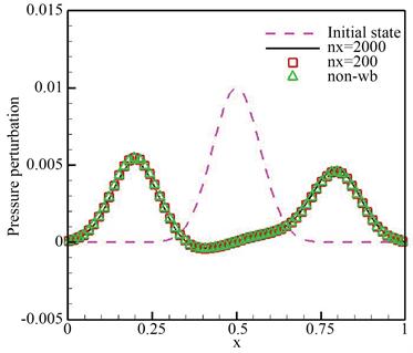
3.3. 等温气体的小扰动问题

本算例的目的在于通过对等温气体的小扰动来检验well-balanced方法的优点，这个算例借鉴LeVeque [27] 提出的算例，且在文献 [28] [29] [30] 中也采用过。管道高度在x截面上为 $h\left(x\right)=\frac{1}{g}x$ 定常状态如下：

${\rho }_0\left(x\right)=p_0\left(x\right)=\exp \left(-x\right),u_0\left(x\right)=0,$ (21)

计算区域为 $\left[0,1\right]$。我们设定初始密度和速度为定常状态(21)，但是针对压力施加一个小扰动

$p\left(x,0\right)=p_0\left(x\right)+\eta \exp \left(-100{\left(x-0.5\right)}^2\right),$

其中 $\eta$ 表示扰动参数。在这里，分别考虑两个扰动参数 $\eta =0.01$ (大脉冲)和 $\eta =0.0001$ (小脉冲)。我们使用100个单元将该算例计算至时刻 $t=0.2$，并与通过2000个单元得到的参考解相比较。压力扰动分别如图1所示，为了方便比较，我们还给出了non-well-balanced方法的数值结果(用“”)。

(a) $\eta =0.01$ (b) $\eta =0.0001$

Figure 1. Numerical results of the example in Section 3.3 by the well-balanced method (denoted by “”) and by the non-well-balanced method (denoted by “”)

图1. 在3.3节例子的well-balanced方法(用“”表示)与non-well-balanced方法(用“”表示)的数值结果

很明显，相关扰动分裂成两个方向相反的波，并且在最后时刻脉冲振幅减小。对于两个脉冲，well-balanced方法生成的数值结果均与参考解很好地匹配，且不存在伪振荡。与此同时，non-well-balanced方法只能对大脉冲产生良好的效果，而不能有效捕获小脉冲，同时存在伪振荡。

3.4. 引力场下的一维激波管问题

在本节中，我们模拟标准Sod问题 [31] [32] [33] 来验证well-balanced方法的能力，该算例涉及到快速变化的激波、接触波和稀薄波。间断初始条件如下

$\left(\rho ,u,p\right)\left(x,0\right)=\{\begin{array}{l}\left(1,0,1\right),如果x\le 0.5\\ \left(0.125,0,0.1\right),否则,\end{array}x\in \left[0,1\right]$

截面高度取作 $h\left(x\right)=\frac{1}{g}x$，参数分别取作 $R=480$， $\theta \left(x\right)={\theta }_{ext}=288.15$。我们将数值结果展示与图2，可以很明显地看出，所设计方法生成的数值结果拥有非常高的分辨率，且保持陡峭的间断过渡，这从侧面显示了方法的优势。

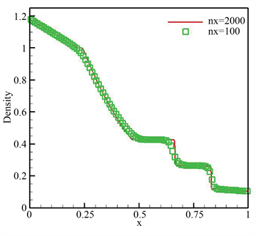(a) 密度 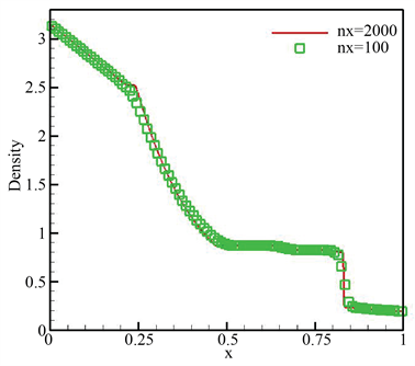(b) 能量 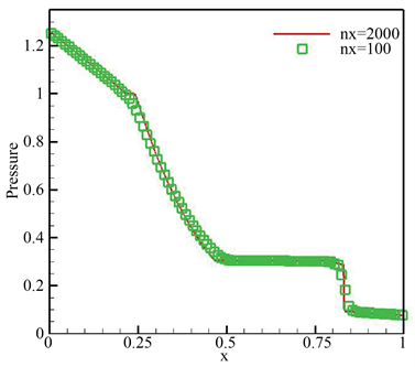(c) 压力 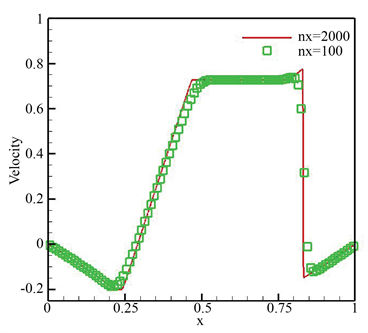(d) 速度

Figure 2. Numerical results of the example in Section 3.4 at t = 0.2

图2. 第3.4节例子在t = 0.2时的数值结果

4. 结论

在本文中，我们针对管道中天然气流动模型开展了高精度方法的研究工作。该模型可经由带有源项的欧拉方程来刻画。我们针对此模型构造了高阶well-balanced DG方法。首先，将原始控制方程表示为等价形式，使得我们能够更方便地构造well-balanced数值流通量。然后，借助一种新颖的源项离散，得以精确保持针对流通量梯度的离散和源项离散二者之间的平衡。严格的理论分析以及广泛的数值结果均表明，本方法保持well-balanced性质。更进一步，该方法针对光滑解保持高阶精度，基于相对粗网格可以有效捕捉针对定常状态的小扰动，并且对于间断解保持陡峭的间断过渡。

致谢

本研究得到了国家自然科学基金面上项目(No. 11771228)的资助。

NOTES

^*通讯作者。